
Summarize Data with Advanced Filter
April 11, 2018 - by Bill Jelen

Your manager needs a summary of total revenue, cost, and profit for each customer in a large data set. Today I look at Advanced Filter and SUMIF to solve the problem.
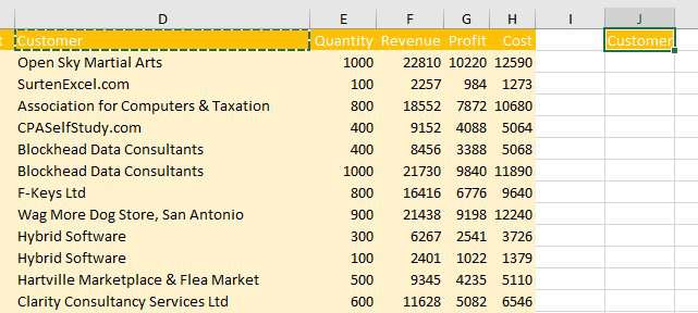
The goal is to summarize this 563-row data set so you have one row per customer.
This week will feature five different ways to solve the problem.
- Monday: Summarize Data with Subtotals
- Tuesday: Summarize Data with Remove Duplicates
- Today: Summarize Data with Advanced Filter
- Thursday: Summarize Data with Consolidate
- Friday: Summarize Data with Pivot Tables
- Saturday: Summary of Summarize Data Week
Watch Video
Video Transcript
Learn Excel from MrExcel Podcast, Episode 2189: Summarize with Advanced Filter.
Hey, welcome back to the MrExcel netcast, this is Summarizing Data week. This is our third method; we're trying to create a summary of 1 row per Customer. So far, we used Subtotals and Remove Duplicates. I'm going to go old school here: Copy these headings over to an output range and use Advanced Filter.
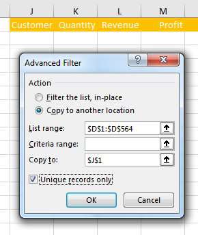
Now, my Advanced Filter is just going to be on column D like this. So that was Ctrl+Shift+Down Arrow, choose Advanced, Copy to another location-- where am I going to copy it to? That heading in J. And then, right here, "Unique records only". This was long before we had to Remove Duplicates, would get us a unique list of customers like that. Alright, now that we have this list of customers we have to build a formula.
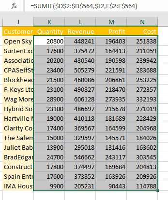
Yesterday, I used SUMIFS, today I'll try SUMIF. And what we do is, we say we're going to look through all those Customers over in column D. So, from here, Ctrl+Shift+Down Arrow, press F4 to put the dollar signs in; comma, then the criteria is here in J2-- click on J2-- press F4-- 1, 2-- 3 times; single dollar sign before the J; and then, finally, where are the numbers coming from? Well, they're coming from the quantity column-- so, here, Ctrl+Shift+Doen Arrow, and I'll press F4-- 1-- 2 times to lock it down to just the columns like that; and then Ctrl+Enter. Once we have that first formula in, drag across, double-click the Fill handle to shoot it down, and there's our results.
All these methods are in this new book, MrExcel LIVe, The 54 Greatest Tips of All Time. Click that "I" on the top right-hand corner to check out more about the book.
This week-- all this week-- we're doing a series on Summarizing Data. So far, we've done Subtotals, Remove Duplicates, today Advanced Filter. How to summarize with Advanced Filter: Copy the headings to an output range; select Data in the Customer column; Data, Filter, Advanced, Copy to another location; specify that Customer heading as the output; "Unique items only"; click OK; then it's a simple SUMIF formula; and copy that down.
Hey, I want to thank you for stopping by, we'll see you next time for another netcast from MrExcel.
- Copy the headings from D1:H1 and paste to J1. The J1 will become the Output range. K1:M1 headings will be used later.
- Select D1. Press Ctrl + Shift + Down Arrow to select to the end of the data.
- Select, Data, Advanced Filter. Choose Copy to Another Location. The List Range is correct. Click in Copy To: and click on J1. Choose the box for Unique Items Only. Click OK.
- Select K2. Ctrl + Shift + Down Arrow and Ctrl + Shift + Right Arrow to select all of the numbers.
-
Enter a formula of
=SUMIF($D$2:$D$564,$J2,E$2:E$564). Press Ctrl + Enter to fill the selection with a similar formula
After 37 clicks, you have this result:
This method is similar to Adam's method from Tuesday. Entering the formula requires a lot of keystrokes. Tomorrow, an ancient method that will dramatically reduce keystrokes.
This week is Summarizing Data week. Each day, we will look at five different ways to solve a problem.
Excel Thought Of the Day
I've asked my Excel Master friends for their advice about Excel. Today's thought to ponder:
“Excel is the second best software in the world” [for anything]
Title Photo: Nathan Numlao / Unsplash