Sum Every Other Row or Every Third Row
January 27, 2021 - by Bill Jelen

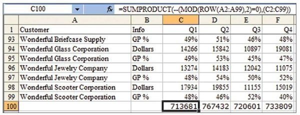
Challenge: In Figure 7, someone set up a worksheet with dollars in rows 2, 4, 6, 8, and so on and percentages in rows 3, 5, 7, 9, and so on. You want to sum only the dollars, which are stored in the even rows. While you’re at it, you’d like to know how to sum the odd rows or every third row.
Solution: There are a lot of possible approaches to this problem, some of which require you to figure out which rows to sum.
- To sum the odd rows:
=SUMPRODUCT(MOD(ROW(3:100), 2), (C3:C100)) - To sum the even rows:
=SUMPRODUCT(--(MOD(ROW(2:99), 2)=0), (C2:C99))or=SUMPRODUCT(MOD(ROW(1:98),2), (C2:C99)) - To sum every third row (2, 5, 8, etc.):
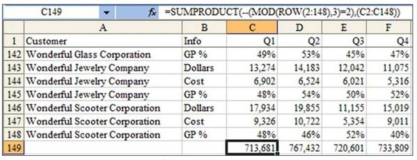
=SUMPRODUCT(--(MOD(ROW(2:148),3)=2), (C2:C148)). See Figure 8

Summing the Odd Rows
Think back to when you were just learning division. If you had the problem 38 divided by 5, you would write that the answer is 7 with a remainder of 3. Excel
provides the MOD function to return the remainder in a division problem. – For example, =MOD(7,2) calculates 7 divided by 2 and returns 1 as the remainder. The remainder of an odd number divided by 2 is 1. It is 0 for all even numbers. You can therefore use MOD to assign a 1 to each odd-numbered row and a 0 to each even-numbered row.
The problem is simple if you want only the odd rows. You can use an array of 1s and 0s in SUMPRODUCT. Multiplying the range C3:C100 by the result of the MOD function (an array of alternating 1s and 0s) results in every other number being added up.
Summing the Even Rows
The MOD(ROW(),2) function returns 1 for an odd row, and it returns 0 for an even-numbered row. Therefore, if the result of the MOD function is 0, you know you’re working with an even-numbered row. Using MOD(ROW(),2)=0 will return an array of TRUE and FALSE values. You can then use the double minus sign to convert the TRUE/FALSE values to 1/0 values.
A simpler but less intuitive solution is to adjust the MOD argument so that it is one row behind the sum range. If you hope to grab the even rows from C2:C99, you can specify a range for the ROW function that starts one row above the real range. Use MOD(ROW(1:98),2) to ensure that the first value MOD returns is 1, followed by 0, 1, 0, 1, and so on.
Summing Every Third Row
Figure 8 shows a situation in which cost rows have been added. In this case, you would like to sum every third row—rows 2, 5, 8, etc. If you use =MOD(Row,3), you get 1 for rows 1, 4, and 7. You get 2 for rows 2, 5, and 8. You get 0 for rows 3, 6, and 9. To sum only the sales rows, you need to test if the result of the MOD function is a 2. Since this test will return TRUE/FALSE values, use the double minus to convert the True/False values to 1/0 values. So the formula becomes:
=SUMPRODUCT(--(MOD(ROW(2:148),3)=2, (C2:C148))

Alternate Strategy: While all the solutions presented so far are going to amaze your co-workers, they are all inherently dangerous. If someone inserts a new row in the worksheet, the MOD functions won’t work as you want them to.
It was not stated in the original problem, but if the worksheet really has a column B that identifies Dollars and GP%, then it would be safer to use a SUMIF function to sum the dollar amounts:
=SUMIF($B2:$B99, "Dollars", C2:C99)
This formula instructs Excel to look through B2:B99. If the value in that row says “Dollars”, Excel adds up the corresponding value from column C. With this solution, there is no worry that dollars on even rows will accidentally shift to odd rows.
Summary: While you can guru-out with SUMPRODUCT solutions galore, the simplest solution might be to use SUMIF.
Source: "Add every other row" on the MrExcel Message Board.
Title Photo: Fran at Unsplash.com
This article is an excerpt from Excel Gurus Gone Wild.
