Sort Subtotals
April 14, 2021 - by Bill Jelen

Challenge: You want to chart the sales for the five largest customers in a data set.
Solution: You can sort the collapsed view of a subtotaled data set. Here’s how:
- Choose one cell in the customer column. Click the AZ button to sort in ascending order.
- Choose Data, Subtotals. In the Subtotal dialog box, change the At Each Change In dropdown to Customer. Make sure the Use Function dropdown is Sum. Choose at least the Sales column from the Add Subtotal To section. Click OK. Excel adds subtotals for each customer.
- Look at the left of column A. Excel has added three group and outline buttons, labeled 1, 2, and 3. Click the 2 button to see one line per customer.
- Choose one cell in the Sales column. Click the ZA button to sort the largest customers to the top of the list.
- Select cell A1 through the fifth customer total. In Excel 2003, press F11 to create a chart. In Excel 2007, press Alt+F1 to create a chart on the current page.
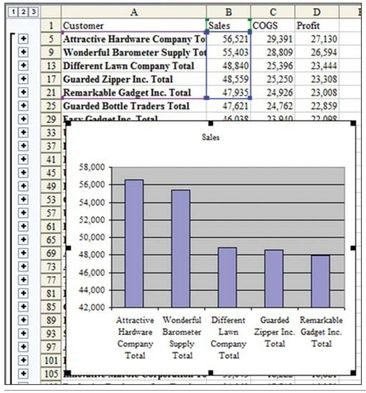
As shown in Figure 69, Excel creates a chart of the five largest customers.

Breaking It Down: There are two amazing features here. First, you can successfully sort a subtotaled data set when it is in the collapsed state. Excel actually rearranges groups of rows while doing the sort. (Each group contains the hidden detail rows for one customer and the visible subtotal row.) Second, in step 5, you take advantage of the fact that charts by default hide data that is hidden in the worksheet. Although your selection might include rows 1 through 21, the chart shows only the visible subtotals in rows 5, 9, 13, 17, and 21.
Summary: Excel properly sorts data when you’ve collapsed the view to show only the subtotals. After you sort the data to find the five largest customers, you can use Excel to create a chart based on the data.
Title Photo: Alex Block on Unsplash
This article is an excerpt from Excel Gurus Gone Wild.
