Sort or Filter by Icon
October 16, 2017 - by Bill Jelen

You have Excel data with icons, such as traffic lights. You want to find all of the red icons. You can sort or filter by color.
Conditional formatting got a lot of new features in Excel 2007, including icon sets and more than three levels of rules. This allows for some pretty interesting formatting over a large range. But, once you format the cells, you might want to quickly see all the ones that are formatted a particular way. In Excel 2007, sorting and filtering were also updated to help you do just that!
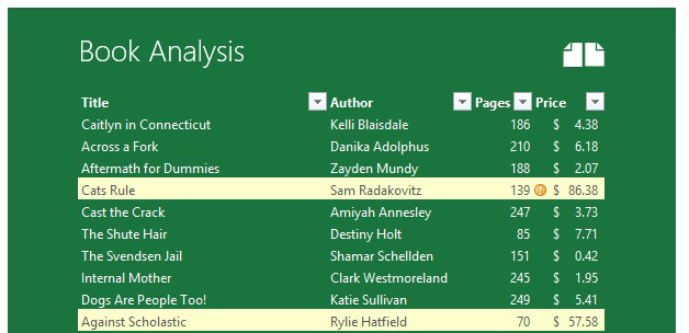
This book analysis table has some highlighted rows to flag interesting books and an icon next to the price if the book is in the top 25% of prices in the list:

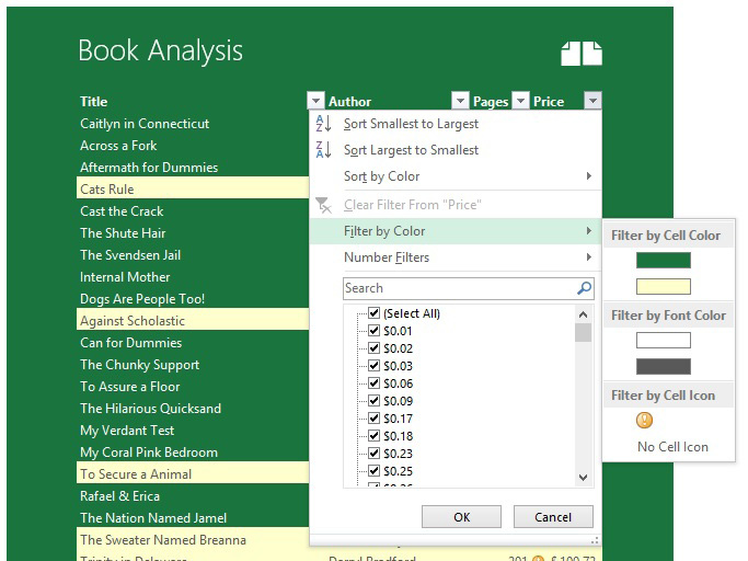
If you want to quickly view all the highlighted rows or cells that have icons, just dropdown the filter for the column and choose Filter by Color (or Sort by Color to bubble them to the top):
Then you can pick the formatting you want to sort or filter by! This doesn’t just work for conditional formatting; it also works for manually coloring cells. It is also available on the right-click menu of a cell under the Filter or Sort flyout, and in the Sort dialog.

This tip is from Sam Radakovitz, a project manager on the Excel team. He is more fond of cats than dogs.
Watch Video
- Today's trick is from Sam Radakovitz on the Excel team
- Sam's signature formatting is white Segoe UI on Excel Green RGB(26,116,61)
- Creating your own icon set to show items in top 25%
- Creating a formula-based conditional formatting to highlight entire row
- Use Filter dropdown to filter by color or by icon
- Right-click to filter by color or icon
- Right-click to sort by filter or icon
- Idea to allow filtering by two colors
- Vote at mrx.cl/filtertwocolors
Video Transcript
Learn Excel from MrExcel podcast, episode 2049 – Sort, or Filter, by Icon!
I am podcasting all of the tips in this book, click that “i” in the top-right hand corner to subscribe to the playlist.
Alright, today's tip is from Sam Rad, Sam Radakovitz is on the Excel team, and one thing I love from Sam is the way his sheets look cool all the time. I always go to school and try and learn how Sam is doing this, and one Of Sam's signature moves here is Segoe UI as the font, that white on this green background. What is this green? We have to come here to More Colors and Custom, and that's the magic Excel green, 26-116-61. So if you want to start creating worksheets that look like Sam's, you can start using those formats, they always look really, really cool.
Alright, so Sam was talking about Sort and Filter by Icon, and he actually created a really cool icon set here, where he looked at things in the top 25% of price. So we'll select all of those cells, and then go to Home, Conditional Formatting, Icon Sets, and choose a 4-level icon set, really important that he uses 4 levels, alright, so that gets that default. And then we wanted a conditional formatting and manage the rules, and then Edit that Rule, and Sam's goal is to highlight things at the top 25%. So by using 4 icons, it's automatically set up at the right levels, great tip there, and then No Cell Icon, No Cell Icon, No Cell Icon, and then for this one, he chose this nice yellow exclamation point, right? So, you don't have to use the sets that are building, you can build your own sets, or in this case I use a set to highlight just things that are in the top 25%, that's cool.
The other thing that Sam did, is a great trick that I've done before, to highlight the entire row. So Sam's going to use a formula here, Conditional Formatting, create a New Rule, use a formula to determine which cells to format. And you know, we are currently sitting in cell C4, so this formula has to work from the point of view of C4, but it has to be able to be copied throughout. So we're going to look for everything where the price in F, so $F4, that's really important! We always want to look in F, but the 4 is allowed to move, as it gets copied down, divided by the page count in E is > let's say $10c a page, and we'll just format that. I will go back to the Fill color here, go to More Colors, choose this nice light yellow, and then change the font for these two, maybe black, click OK, click OK, click OK. Alright see, THAT is cool, because that highlights the entire row for something based on a calculation over here in E and F.
Alright, now, so now that we've applied these, if we want to look at the things highlighted with the icon or highlighted with the color, we can turn on the filters. So Data, Filter, and you can open this dropdown, and under Filter by Color, we can either filter to all of the things that have the yellow color, I'll undo that. Or we can right-click and go to Filter and say “Filter by Selected Cell’s Icon”, and we'll be able to quickly filter to everything that is both yellow, or has the exclamation point. So either right-click or using the drop-down. Now, let's turn the filters off, it's also possible to come in here and sort, alright. So if we want to sort all of that icon to the top, we just choose a cell, right-click and say Sort, Put Selected Cell Icon on Top, and we can pull all of those items to the top of the list. Alright, these are great techniques.
Alright now, I'm going to deviate from Sam’s trick here, and actually, unfortunately, makes it more work for Sam. You know, when we use filters, one of the nice things that got added to Excel 2010 is the ability to search, alright. So we want to search for all books that have word “dog”, it finds all those and that works great, that's awesome, right? But then we could also come back in here, and search for all books that have the word “cat”, and then this beautiful thing called Add current selection to filter, click OK, and we now have a list of all of the items that are either dog or cat.
Alright, so that's a cool bit of functionality that I really like, but I was doing an Excel seminar yesterday in Nashville. And someone pointed out that if you want to filter by color, if you needed a filter to everything that's green or yellow, there is no equivalent ability to select multiple items, you can't click here and drag or anything like that, alright. I said “Oh, you're right, I've never tried to do this!” but if this is something you have to do, I can see where it would be a frustrating thing.
So I went out to excel.uservoice.com and sure enough there's already someone there, go to mrx.cl, that's a country of Chile domain there, /filtertwocolors, and you end up out here where Arne has suggested like to be able to filter columns by more than one color, alright? I already voted, I think you should go out and vote, we want to get at least 20 votes here, that way the Excel team can take a look at this idea. Alright, well hey, it's Friday, that means for half the world it's payday, just $10 for this book, the e-book, or $25 in print, click that “i” on the top-right hand corner. Now we're almost done with the book, I sure would appreciate if you'd buy this book to get a quick recap of the last 70 podcasts.
Alright, today's trick from Sam Rad on the Excel team, talked about Sam's signature formatting white Segoe UI font on the Excel green RGB 26-116-61. Created our own icon set to show items at the top 25%, remember, started out with 4 icons, and then changed the lower 3 to No Cell Icon. And then created a formula-based condition to highlight the entire row. We use the filter dropdown to filter by color, or by icon. You can also right-click to filter by color icon, or right-click to sort by filter icon, and then asked you to vote for that idea to allow filtering by two colors. Go ahead and vote there at mrx.cl/filtertwocolors!
I want to thank you for stopping by, we'll see you next time for another netcast from MrExcel!
Download File
Download the sample file here: Podcast2049.xlsm
Title Photo: traveLink / Pixabay
