Show Yes/No in a Pivot Table

December 12, 2022 - by Bill Jelen

Problem: I want to show Yes/No values in a pivot table. If the customer bought from us in a period, show Yes. If there were no sales, show No.

With dates in the Row field, choose the first date in the pivot table. — Figure 856. Instead of numbers, show Yes/No.

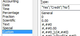
Strategy: Use a custom number format of “Yes”;”Credit”;”No”. Follow the steps in “Specifying a Number Format In a Pivot Table”. Once you are in the Format Cells dialog for the Sum of Revenue field, choose Custom and type the code, including the quotes.

In the Custom box, type "Yes";"Credit";"No" — Figure 857. Show Yes for any positive value, No for zero.

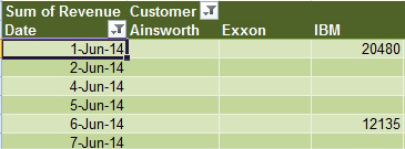
Gotcha: This trick initially shows Yes for periods where there is a purchase, but leaves the other periods blank.

The "Yes" values appear in the pivot table, but the other values are empty. — Figure 858. The Yes values appear.

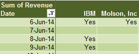
To display the No values, you have to replace the blanks in the pivot table with a zero. See “Replace Blanks in a Pivot Table with Zeroes.”

In Pivot Table Options, choose For Empty Cells Show: 0. — Figure 859. Replace blanks with zero.

Result: The pivot table shows Yes or No values.

The Values area of the pivot table now says Yes or No. — Figure 860. Instead of numbers, show Yes/No.

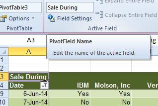
Additional Details: At this point, the heading of “Sum of Revenue” is not really appropriate. Select any Yes/No cell to make the active field box in the Analyze tab of the ribbon say Sum of Revenue. You can type a new name in that box.

Select a cell in the pivot table and then type a new name in the PivotField Name box (it is just above the Field Settings button). — Figure 861. Change from “Sum of Revenue”.

This article is an excerpt from Power Excel With MrExcel

Title photo by Ana Municio on Unsplash