Show Customer Account & Name


January 31, 2023 - by

Show Customer Account & Name

Problem: My source data comes from the sales reps. They don’t use consistent names, so I end up with multiple customer names for one account number.
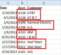
A sloppy customer field shows that Account A128 is both AT&T (without spaces) and AT & T (with two spaces).  Account A398 is both General Electric and G.E. Account A533 is IBM (no spaces) and I B M (with spaces after the I and B. Account A911 is both Wal*Mart and Wal-Mart.
Figure 984. Bad for pivot tables.

This forces me to put both Acct and Customer in the row area. This looks horrible. The customer name doesn’t appear on the totals for each account.
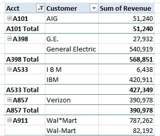
When you put both Account and Customer in the Rows area of a pivot table, both spellings of these customers are on a different row. With Sum of Revenue in column C, you can tell which spelling is used more often. For example, General Electric had $540K in purchases and the G.E. abbreviation had 27,932 in sales.
Figure 985. You want Acct and Customer on the total row.

Strategy: This common problem would be solved if the Excel team would allow you to add Customer Name to the pivot table with a calculation of “First” or “Last”. Look; we don’t really care if we get G.E. or General Electric…either one is a million times better than an empty cell on the total row.


But, for now, we don’t have First or Last. Your best bet is likely to be creating a pivot table with Acct and Revenue. Copy the entire pivot table. Paste as Values.
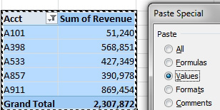
A pivot table with only Account and Revenue is copied. The Paste Special dialog is showing Values.
Figure 986. Convert the pivot table to values.


You are now allowed to insert a blank column between Acct and Revenue. Use a VLOOKUP back into the original data set to fill in the customer name.
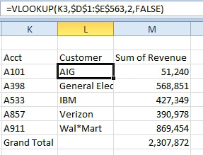
After converting the pivot table to Values, insert column B with a heading of Customer. Use a VLOOKUP to retrieve the first customer name for that account from the original data. The formula for row 3 is =VLOOKUP(K3,$D$1:$E$563,2,False)
Figure 987. Use a VLOOKUP to get the text fields.

Alternate Strategy: You can do the FIRST yourself back in the original data set. Add a column called Acct - Customer. Use a formula to concatenate the Acct with a VLOOKUP to return the first customer from the list.
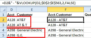
A different solution: In the original data set, you have Account in D and Customer in E. Add a Account-Customer column that concatenates =D2 & "-" & VLOOKUP(D2,$D$2:$E$563,2,False).
Figure 988. Build your own Acct-Customer field.

When you build the pivot table, put this field in the row labels.
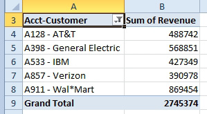
Now, the Pivot Table shows Account - Customer in column A. There are less extra rows:
A128 - AT&T
A398 - General Electric
A533- IBM
Figure 989. This has the data that you need and avoids the duplicate customer names.

This article is an excerpt from Power Excel With MrExcel

Title photo by Skye Studios on Unsplash