See Detail Behind One Number in a Pivot Table

November 25, 2022 - by Bill Jelen

Problem: One number in my pivot table seems to be wrong. Air Canada does not typically buy XYZ, yet it is shown with that product in the report.

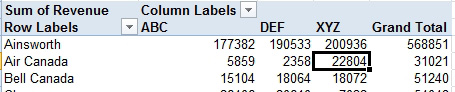
Strategy: You can see the detail behind any number in a pivot table by double-clicking on the number. Click on the $22,804 for Air Canada XYZ. A new worksheet is inserted to the left of the current sheet, showing all the records that make up the $22,804.

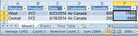
Additional Details: If you double-click on a number in the total row or total column, you will see all the records that make up that number. You could even drill down on the Grand Total cell to get a copy of all the original records.

Gotcha: Each drill-down creates a new worksheet. The new worksheet is just a snapshot in time of what made up the original number. If you detect a wrong number in the drill-down report, you need to go back to the original data to make the correction.

This article is an excerpt from Power Excel With MrExcel

Title photo by Sam Schooler on Unsplash