
Run Many Pivot Tables From one Slicer
January 11, 2023 - by Bill Jelen

You can already see that slicers are better than Report Filters. Another major advantage is that you can filter many pivot tables from one set of slicers. This allows you to create dashboard-like reports.
When you create a pivot chart, the pivot table and chart are placed next to each other by Microsoft. They absolutely do not have to stay next to each other. You can build four pivot charts, each on their own sheet, then move the charts so that they are all on the same worksheet. You can move a chart using the Move Chart icon on the Design tab, or simply select the chart, cut, then paste in a new location.
Here is the process for making the slicers drive all of your pivot tables:
1. Build the first pivot table or pivot chart. Add slicers to that pivot table.
-
2. Build additional pivot tables or pivot charts. Move the chart or table to be near the first pivot table.
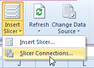
3. While the second pivot table is selected, go to the Analyze tab. Open the dropdown attached to the Insert Slicer icon and choose Slicer Connections. (If you have a Pivot Chart, the Slicer icon is on the Analyze ribbon tab.)
4. Repeat steps 2 & 3 for each additional pivot table or pivot chart.
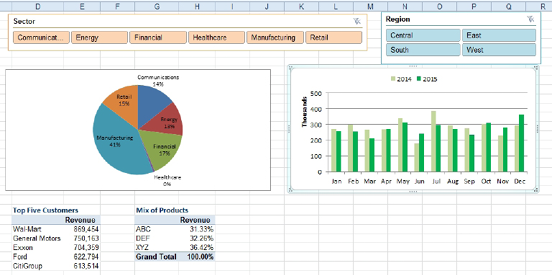
Below, slicers are driving two pivot charts and two pivot tables.
Filter Dates Using a Timeline in Excel 2013 & Newer
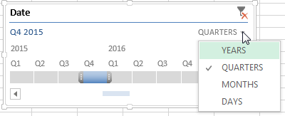
Excel 2013 introduced a new type of filter called a Timeline. It only works for date columns. You can choose to filter by Day, Month, Quarter, or Year.
You can run many pivot tables from one Timeline.
This article is an excerpt from Power Excel With MrExcel
Title photo by Dave Hoefler on Unsplash