Return Data from a Webservice

July 25, 2022 - by Bill Jelen

Microsoft introduced three new functions in Excel 2013 that will return data from a webservice.

You will use at least two of the functions in conjunction with each other.

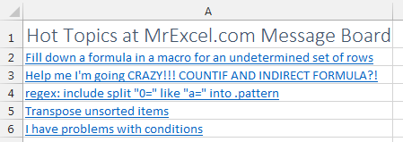
The first thing to do is to find a URL that returns data from a webservice. In this example, I am using https://feeds.feedburner.com/MrexcelExcelForumTop10Posts. This will return the five hot topics from the MrExcel Message board.

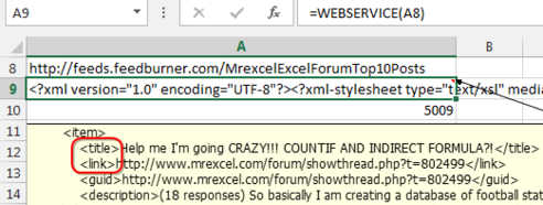
In my example, I enter (or use formulas to build) the webservice address in cell A8.

In cell A9, I use the formula =WEBSERVICE(A8). This formula reaches out to the web and returns a massively long result to cell A9. In my case, it returns 5009 characters of XML.

I hate to characterize the stuff in A9 as gobbledegoo. It is certainly machine readable and harder for humans to understand. But, if you copy A9 and paste to Notepad or to a text box, you will start to see some patterns. For me, I can tell that I want a field called “title” and another field called “link”.

Because I am already familiar with this data source, I know there are generally five topics returned. However, there are some headers, so there are 7 occurrences each of title and link in the 5009 characters returned by the WEBSERVICE function.

To extract the titles to a range in Excel, follow these steps:

• 1. Select seven vertical cells. In my case, A12:A18.

• 2. Type =FILTERXML(A9,”//title”). This is something called XPATH. I won’t claim to know anything about XPATH, but putting two slashes and the field name seems to do the trick.

• 3. Because you want this one formula to return 7 values, do not press Enter to accept the formula. Instead, hold down Ctrl+Shift and then press Enter. Excel will return all 7 titles to A12:18.

Those steps required some trial and error. I initially only selected five cells, then noticed the two headers were being returned. So, I cleared those formulas and tried again with 7. I might have tried again with 8, but then the 8th value would have retuned #N/A.

Over in B12:B18, the array formula is =FILTERXML(A9,”//link”).

To put it all back together in a nice report, I use =HYPERLINK(B14,A14) in cell A2 and copy down five cells.

There is one more function that you might use - it is called ENCODEURL. Imagine that you are allowing someone to select a city from a dropdown list. They select the city. You use VLOOKUP to return the correct city code and then concatenate the whole thing together into a URL. If there is any chance that the result will contain an illegal character, you can wrap the formula in ENCODEURL to convert those illegal characters into a valid URL.

This article is an excerpt from Power Excel With MrExcel

Title photo by Shannon Potter on Unsplash