
Replacing VLOOKUP using the Data Model and Relationships
March 07, 2018 - by Bill Jelen

Don't have Power Pivot? Doesn't matter. Most of Power Pivot is built in to Excel 2013 and even more in Excel 2016. Today, our tip from Ash is joining tables in a pivot table.
Every Wednesday for seven weeks, I am featuring one of the favorite tips from Ash Sharma. Ash is a product manager on the Excel team. His team brings you pivot tables and many other good things. Today, Ash's favorite feature is joining multiple data sets using Relationships and the Data Model.
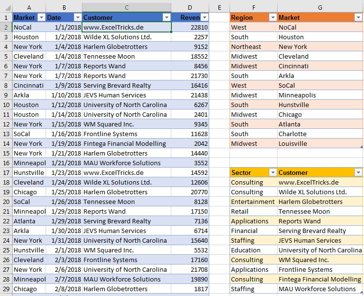
Say that your I.T. department gives you the data set shown in columns A:D. There are fields for customer and market. You need to combine certain markets into regions. Each customer belongs to a sector. Region and Sector are not in the original data, but you have lookup tables to provide this information.
VLOOKUPs are powerful. But the Data Model is so much simpler.
Normally, you would flatten the data by using VLOOKUP to pull data from the orange and yellow tables in to the blue table. But since the key field is not on the left side of each table, you will either have to switch to INDEX and MATCH, or re-arrange the lookup tables.
Starting in Excel 2013, you can leave the lookup tables where they are and combine them in the pivot table report itself.
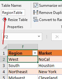
For this technique to work, all three tables must be Formatted as a Table. Select one cell in each data set and choose Home, Format as Table or press Ctrl + T. The three tables will initially be called Table1, Table2, and Table3. I use the Table Tools Design tab of the Ribbon and re-name each table. I also change the color of each table. In this example, the blue table is called Data. The orange table is RegionTable. The yellow table is SectorTable.
Note
Some will tell you that you should use geeky names like Fact, TblSector and TblRegion. If anyone hassles you like this, just steal their pocket protector and let them know that you prefer English-sounding names.
To rename a table, type a new name in the box on the left side of the Table Tools Design tab. Table names should not have spaces.
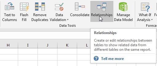
Once the three tables are defined, head to the Data tab and click on Relationships.
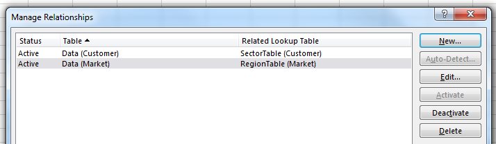
In the Manage Relationships dialog, click New. In the Create Relationship dialog, specify that the Data table's Customer field is related to the SectorTable's Customer Field. Click OK.
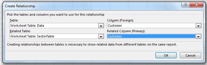
Define another new relationship between the Market field in the Data and RegionTable fields. After defining both relationships, you will see them in the Manage Relationships dialog.
Congratulations: you have just built a Data Model in your workbook. It is time to build a pivot table.
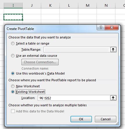
Select the blank cell where you want your pivot table to appear. By default, the Create PivotTable dialog will choose Use This Workbook's Data Model. The pivot table location will default to the cell that you chose. Click OK.
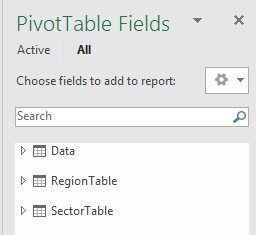
The Pivot Table Fields list will list all three tables. Use the triangle to the left of a table to expand the table name to show you the fields.
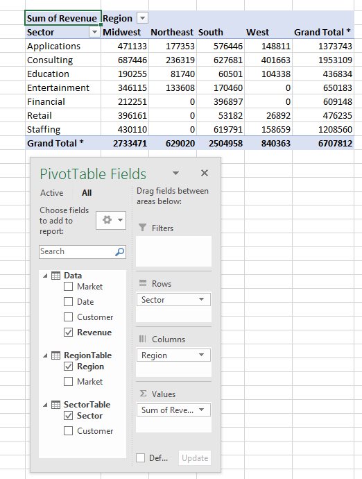
Expand the Data table. Select the Revenue field. It will automatically move to the Values area. Expand the SectorTable. Choose the Sector field. It will move to the Rows area. Expand the RegionTable. Drag the Region field to the Columns area. You will now have a pivot table summarizing data from the three tables.
Note
In every book that I've written before today, I use a different technique to build this report. After defining the three tables, I choose cell A1 and Insert, Pivot Table. I check the box for Add This Data to the Data Model. In the Pivot Table Fields list, select All from the top of the list. Choose fields for the report, and then define the relationships after the fact. The technique described above seems smoother and actually involves a tiny bit of planning ahead. The people who use Option Explicit in their VBA code would definitely like this method.
The relationships in the data model make Excel feel more like Access or SQL Server, but with all of the goodness of Excel.
I love to ask the Excel team for their favorite features. Each Wednesday, I will share one of their answers. Thanks to Ash Sharma for supplying this idea.
Excel Thought Of the Day
I've asked my Excel Master friends for their advice about Excel. Today's thought to ponder:
"Don’t lookup if you’re in a relationship"
Title Photo: Geralt / Pixabay