Replaced Nested IF with VLOOKUP
September 19, 2017 - by Bill Jelen

Do you have an Excel formula that nests multiple IF functions? When you get to the point with too many nested IF statements, you need to see if the whole thing would become simpler with a simple VLOOKUP function. I've seen 1000-character formulas be simplified to a 30-character VLOOKUP formula. It is easy to maintain when you have to add new values later.
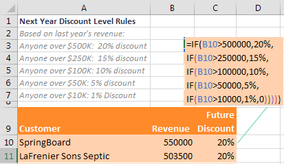
A long time ago, I worked for the vice president of sales at work. I was always modeling some new bonus program or commission plan. I became pretty used to commission plans with all sorts of conditions. The one below is pretty tame.
The normal approach is to start building a nested IF formula. You always start at either the high end or the low end of the range. “If sales are over $500K, then the discount is 20%; otherwise….” The third argument of the IF function is a whole new IF function that tests for the second level: If sales are over $250K, then the discount is 15%; otherwise,...”
These formulas get longer and longer as there are more levels. The toughest part of such a formula is remembering how many closing parentheses to put at the end of the formula.
Mini Bonus Tip
Matching the Parentheses
Excel cycles through a variety of colors for each new level of parentheses. While Excel reuses the colors, it uses black only for the opening parenthesis and for the matching closing parenthesis. As you are finishing the formula below, just keep typing closing parentheses until you type a black parenthesis.

Back to the Nested Formula Tip
If you're using Excel 2003, your formula is already nearing the limit. Back then, you could not nest more than 7 IF functions. It was an ugly day when the powers that be changed the commission plan and you needed a way to add an eighth IF function. Today, you can nest 64 IF functions. You should never do this, but it is nice to know there is no problem nesting 8 or 9.
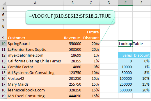
Rather than use the nested IF function, try using the unusual use for the VLOOKUP function. When the fourth argument of VLOOKUP changes from False to True, the function is no longer looking for an exact match.
Well, first VLOOKUP tries to find an exact match. But if an exact match is not found, then Excel settles into the row just less than what you are searching for.
Consider the table below. In cell C13, Excel will be looking for a match for $28,355 in the table. When it can’t find 28355, Excel will return the discount associated with the value that is just less. In this case, the 1% discount for the $10K level.
When you convert the rules to the table in E13:F18, you need to start from the smallest level and proceed to the highest level. Although it was unstated in the rules, if someone is below $10,000 in sales, the discount will be 0%. You need to add this as the first row in the table.

Caution
When you are using the “True” version of VLOOKUP, your table has to be sorted ascending. Many people believe that all lookup tables have to be sorted. But a table needs to be sorted only in the case of doing an approximate match.
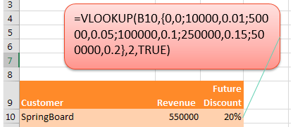
What if your manager wants a completely self-contained formula and does not want to see the bonus table off to the right? After building the formula, you can embed the table right into the formula.
Put the formula in Edit mode by double-clicking the cell or by selecting the cell and pressing F2.
Using the cursor, select the entire second argument: $E$13:$F$18.

Press the F9 key. Excel will embed the lookup table as an array constant. In the array constant, a semicolon indicates a new row, and a comma indicates a new column.

Press Enter. Copy the formula down to the other cells.
You can now delete the table. The final formula is shown below.

Thanks to Mike Girvin for teaching me about the matching parentheses. The VLOOKUP technique was suggested by Danny Mac, Boriana Petrova, Andreas Thehos, and @mvmcos.
Watch Video
- With a tiered commission, bonus, or discount program, you often have to nest your IF functions
- The Excel 2003 limit was 7 nested IF statements.
- You can now nest 32, but I don't think you should ever nest 32
- When would you ever use the approximate match version of VLOOKUP? This is the time.
- Translate the discount program into a lookup table
- VLOOKUP won't find the answer in most cases.
- Putting ,True at the end will tell VLOOKUP to find the value just less.
- This is the only time the VLOOKUP table has to be sorted.
- Don't want the VLOOKUP table off to the side? Embed it in the formula.
- F2 to edit the formula. Select the lookup table. Press F9. Enter.
Video Transcript
Learn Excel from MrExcel podcast, episode 2030 - Replaced Nested IF with VLOOKUP!
I'll be podcasting this entire book, click the “i” on the top-right hand corner to get to the playlist!
Hey, welcome back to the MrExcel netcast, I’m Bill Jelen. Alright, this is really common with either a commission program, or a discount program, or a bonus program, where we have the tiers, different tiers, right? If you're above $10000, you get 1% discount, $50000 5% discount. You have to be careful when you build this nested IF statement, you start it at the top end if you're looking for greater than, or at the bottom end if you're looking for less than. So B10>50000, 20%, otherwise another IF, B10>250000, 25%, and so on and so on. This is just a long and complicated formula, and if your table’s larger, back in Excel 2003, you couldn't nest more than 7 IF statements, we're almost near the limit here. You can go to 32 now, I don't think you should ever go to 32, and even if you're screaming “Hey wait, what about the new function that just came out in Excel 2016, the February 2016 release, with the IFS function?” Yeah sure, there's less parentheses here, and 87 characters instead of 97 characters, it's still a mess, let's get rid of this and do it with a VLOOKUP!
Alright, here are the steps, you take those rules, and you turn them on their head. The first thing we have to say is, if you had $0 in sales, you get a 0% discount, if you had $10000 in sales, you get a 1% discount, if you have $50000 in sales, you get a 5% discount. $100000, 10% discount, $250000, 15% discount, and then finally, anything >$500000 gets the 20% discount, alright. Now lots of times, every time I'm talking about VLOOKUP, I say every VLOOKUP that you ever create is going to end in FALSE, and people will say “Well wait a second, what’s the TRUE version there for anyway?” It's for this very case where we're looking for a range, so we're looking up this value, a regular VLOOKUP, of course, ,2,FALSE will not find 550000, is going to return the #N/A! So in this one very special case we’re going to change that FALSE to a TRUE, and that'll tell Excel “Go look for the 550000, if you can't find it, give us the value that's just less.” So it gives us the 20%, that’s what it does, alright? And this is the only time your VLOOKUP table has to be sorted, all the other times with ,FALSE , it can be however you want. And yes, you could leave the ,TRUE off, but I always put it there just to remind myself that this is one of those weird incredibly dangerous VLOOKUPs, and I don't want to copy this formula somewhere else. Alright, so we'll copy and Paste Special Formulas, alright.
Next complaint: your manager doesn't want to see the lookup table, he wants it “Just get rid of that lookup table.” Alright, we can do that by embedding the lookup table, check this out, great trick that I got from Mike Girvin at ExcelIsFun. F2 to put the formula into Edit mode, and then very carefully select just the range for the lookup table. Press F9, and it takes this table and puts it in array nomenclature, and then I just press Enter like that. Copy that down, Paste Special Formulas, and then I am free to get rid of the lookup table, that all just continues to work down the row. This is a huge hassle if you have to come back in and edit this, you have to really stare at it with lots of clarity. The comma means we're going to the next column, the semicolon means were going to the next row, alright, but you could in theory get back in there and change that formula if one of the chain numbers changes.
Alright, so using a VLOOKUP instead of a nested IF statement is tip #32 on our way to 40, “40 Greatest Excel Tips of All Time”, you can have this entire book. Click that “i” on the top-right hand corner, $10 for an e-book, $25 for the print book, alright. So today we're trying to solve a tiered commission bonus, or discount program. Nested IFs are really common, watch out, 7 is all you can have in Excel 2003, today you can have 32, but you shouldn't ever have 32. So when to use the approximate MATCH version of VLOOKUP, this is it. Take that discount program, turn it upside down, make it into a lookup table starting with the smallest number, and going to the largest number. VLOOKUP, of course, won't find the answer, but by changing the VLOOKUP to ,TRUE at the end, it'll tell it to find the value just less, this is the only time the table has to be sorted. If you don't want to see that table out there, you can embed it in the formula using the Mike Girvin trick, F2 to edit the formula, select the lookup table, press F9, and then Enter.
Alright hey, I want to thank you for stopping by, we'll see you next time for another netcast from MrExcel!
Download File
Download the sample file here: Podcast2030.xlsx
Title Photo: Pixabay
