Replace Blanks in a Pivot Table with Zeros
December 05, 2022 - by Bill Jelen

Problem: When I have no sales of a particular product in a particular region, Excel leaves those cells in the pivot table blank. This seems like a really bad idea. I’ve learned in this book that if my data has blanks instead of zeros, Excel will assume that a column is a text column. It is really ironic that Microsoft would dare to use a blank cell in the middle of numeric results.

Strategy: Follow these steps:
1. Right-click any cell in the pivot table and choose Pivot Table Options.
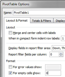
2. In the PivotTable Options dialog, select the Layout & Format tab. You can either uncheck "For Empty Cells Show", or fill in a 0 in the For Empty Cells Show text box. Click OK.

Results: Blanks in the values section of the pivot table are shown as zeros.
Additional Details: You can enter anything in the For Empty Cells Show text box. Some people like to use -- or n.a. in the formerly blank cells. Either works just as well as a zero.
This article is an excerpt from Power Excel With MrExcel
Title photo by Bernard Hermant on Unsplash
