Remove Leading and Trailing Spaces

April 12, 2022 - by Bill Jelen

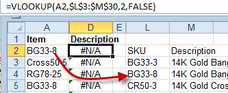
Problem: None of my VLOOKUP formulas are working. I can clearly see that there is a match in the lookup table, but Excel cannot see it.

In this different example, none of the VLOOKUPs are working. In row 2, Excel says there is not a BG33-8 in the table. But a red arrow is pointing to BG33-8. Why can Excel not see the matching part number? — Figure 417. None of the VLOOKUP functions work.

Strategy: A common problem is that either the item in column A or Column L has trailing spaces. This can happen if you downloaded the data from another system.

To fix this problem, you select cell A2 and press the F2 key to put the cell in Edit mode. A flashing insertion cursor will appear at the end of the cell. Check to see if the insertion cursor appears immediately after the last character or a few spaces away.

Edit cell L2 to see if there are trailing spaces. You will likely find that either column has trailing spaces. Below, you can see that there are a couple trailing spaces after the Item in column A. These trailing spaces cause the VLOOKUP to not classify the cells as a match. Although you can tell that “BG33-8 ” is the same as “BG33-9”, Excel cannot.

The BG33-8 in cell A2, now in edit mode. The flashing insertion point is a few spaces after the 8. This data has trailing spaces and those cause the VLOOKUP to not work. — Figure 418. Column A has trailing spaces.

You can use the TRIM function to remove leading and trailing spaces from a value. If there are spaces between words, it will change consecutive spaces to a single space. For example, =TRIM(“ Bill Jelen ”) would change the cell contents to “Bill Jelen”.

Additional Details: If the trailing spaces appear in your lookup value, use TRIM around that one value. Change =VLOOKUP(A2,$L$3:$M$30,2,FALSE) to =VLOOKUP(TRIM(A2),$L$3:$M$30,2,FALSE).

If the trailing spaces appear in the lookup table, then you can actually TRIM the entire table with one bizarre modification. Change the formula above to =VLOOKUP(A2,TRIM($L$3:$M$30),2,FALSE). But, don’t press Enter after making the edit. Instead, hold down Ctrl and Shift and then press Enter.

Gotcha: That formula where you TRIM the entire lookup table is going to be insanely slow. It is fine for impressing your friends who use Excel, but in real life, it would be better to add a temporary column to TRIM each individual cell in column L. Then, copy that column and paste as values over column L.

Alternate Strategy: The other common problem of VLOOKUPs failing is numbers stored as text being used to look up a table with numeric values. Select column A and do Alt+DEF. Repeat with column L. Alt+DEF does a text to columns and converts text numbers to real numbers.

This article is an excerpt from Power Excel With MrExcel

Title photo by Joel Vodell on Unsplash