Quickly Filter a List to Certain Records

September 06, 2022 - by Bill Jelen

Problem: I have 10,000 records in the worksheet. I need to be able to quickly find records that match a criterion, such as all East ABC records.

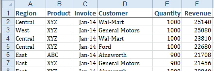
Columns are Region, Product, Invoice, Customer, Quantity, and Revenue. — Figure 666. Find records within this data set.

Strategy: You can find records that match a criterion by using the Filter feature.

Toggle on the Filter command by using either Home, Sort & Filter, Filter or selecting Data, Filter icon. As you can see below, the Filter button is three times larger than the Advanced Filter icon, which I take as evidence that Microsoft someday hopes to add enough power to Filter to eliminate the need for the Advanced Filter.

Click the large Filter icon in the Sort & Filter group of the Data tab. — Figure 667. AutoFilter is now just Filter.

To filter your data set, follow these steps:

1. Make sure your data has a heading row. Select one cell within the data. Select Data, Filter. Excel will add a dropdown to each heading.

Drop-down arrows appear in the right edge of each heading cell: Region, Product, Invoice, and so on — Figure 668. Filter dropdowns.

2. Select the Product dropdown. Before you can select ABC, you have to first uncheck (Select All).

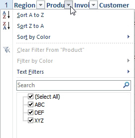
Open the Product drop-down. You can Sort AZ, ZA, by color. A flyout menu offers Text Filters. There is a Search box. Then, checkbpxes next to (Select All), ABC, DEF, and XYZ. — Figure 669. Uncheck Select All, then choose ABC.

3. Click the ABC check box. Click OK. You will now see just the ABC records.
4. Open the Region dropdown. Uncheck (Select All). Check East. Click OK.

You will now have only the East, ABC records. Notice the Funnel icon appears on all columns that have a filter applied.

After filtering to Product ABC, only rows 6, 27, 34, 35, and 44 are shown. The other rows are hidden. It is very subtle, but the drop-down arrow for the Product column changed to a Filter icon to indicate that a filter has been applied to that column. — Figure 670. Excel hides the other rows.

To clear a filter, open the dropdown and choose Clear Filter from Field.

Additional Details: Excel will detect if your column is text, numeric, or dates. Each column type includes a flyout with new options.

The Date filters appear in a tree view, so you can turn on/off entire months rather than clicking all 30 dates that fall in a month. The Date Filter flyout menu offers many choices that seem like they were borrowed from Quickbooks.

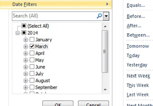
If the column you are filtering contains dates, the Date Filters flyout menu offers Equals, Before, After, Between, Tomorrow, Today, Yesterday, Next Week, This Week, Last week, and others. — Figure 671. Date columns offer many new choices.

Numeric columns offer a Top 10 filter, plus new choices such as Above Average.

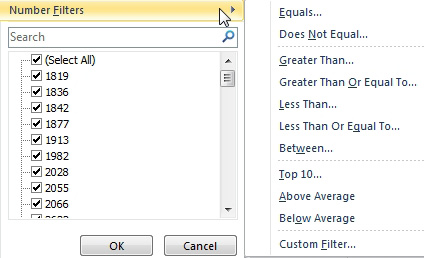
If you are filtering a column of numbers, the Number Filters flyout menu offers Equals, Does Not Equal, Greater than, Greather than or equals to, Less than, Less than or equal to, Between, Top 10, Above Average, Below Average, Custom Filter. — Figure 672. New number filters.

The Top 10 Filter option allows you to specify the top or bottom “n” items or “n%” of items. The Top 10 feature was in previous versions of Excel, but all the other value filters in the figure above are new in Excel 2007.

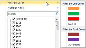
If you have used cell colors, font colors, or icon sets, you can use the Filter by Color fly-out menu to show records that have a certain color.

Open the AutoFilter drop-down and choose Filter by Color. You can either Filter by Cell Color or Filter by Font Color. — Figure 673. Filter by color.

Gotcha: In order for the Date Filters or Number Filters options to appear, your data needs to be predominantly dates or numbers. If you have too many blank cells or too many text cells, Excel will treat the column as text and not offer these filter options in the dropdown.

This article is an excerpt from Power Excel With MrExcel

Title photo by Annie Theby on Unsplash