Preview Remove Duplicates Without Removing Them

October 27, 2022 - by Bill Jelen

Problem: I want to preview which rows will be deleted before deleting them with Remove Duplicates.

Strategy: Use the Formula version of conditional formatting to highlight the cells that will be deleted. Continuing the previous example, say that you want to remove all duplicates of Product+Customer.

Follow these steps:

1. Select A2:H564
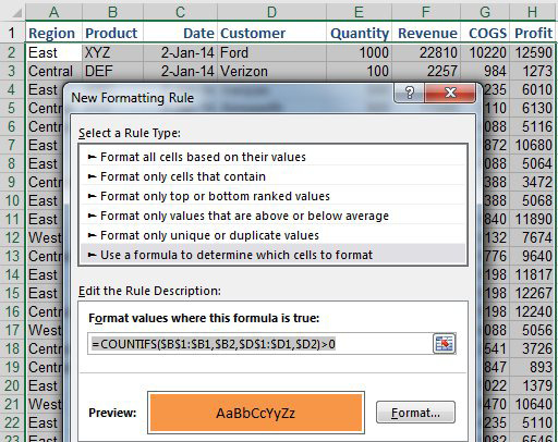
2. Home, Conditional Formatting, New Rule, Use a Formula to Determine Which Cells to Format
3. In the Formula box, type =COUNTIFS($B$1:$B1,$B2,$D$1:$D1,$D2)>0. Note the four references with only a single dollar sign. Those missing dollar signs create an expanding range.
4. Click the Format... button.
5. Choose a Fill color. Click OK once for each open dialog box.

A condtional formating trick to highlight the second (and subsequent) occurences of each customer. This previews what Excel will remove when you use Remove Duplicates. The formula used for Conditional Formatting uses COUNTIF to find all cells above the current cell equal to the customer in B of the current row. If the CountIF is greater than 0, highlight the cell in orange. — Figure 778. The key to this formula are the eight dollar signs.

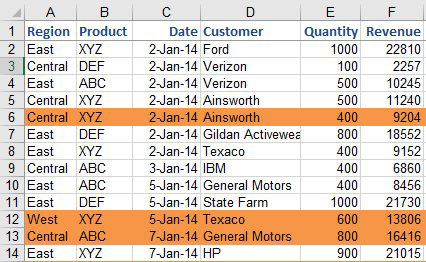
Excel will highlight which rows would be deleted by Remove Duplicates.

The result of the condtional formatting rule. Texaco appears in row 8 and is not formatted. But when Texaco appears a second time in row 12, the whole data row is highlighted with Orange Fill. — Figure 779. Anything highlighted is a duplicate of Product/Customer.

This article is an excerpt from Power Excel With MrExcel

Title photo by pass-° °-Imagination on Unsplash