Power Pivot Portable Formulas
September 01, 2017 - by Bill Jelen

Once you define a new measure in Power Pivot, that formula can be used in subsequent formulas.
If you have the full version of Power Pivot, you can use the DAX formula language to create new calculated fields. From the Power Pivot tab in the ribbon, choose Insert Calculated Field.
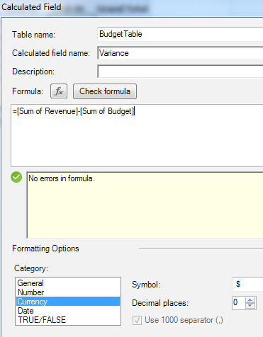
Give the field a name, such as Variance. When you go to type the formula, type =[. As soon as you type the square bracket, Excel gives you a list of fields to choose from.
Note that you can also assign a numeric format to these calculated fields. Wouldn’t it be great if regular pivot tables brought the numeric formatting from the underlying data?
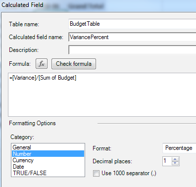
In the next calculation, the VariancePercent is reusing the Variance field that you just defined.
This is great – all of those fields in the pivot table:
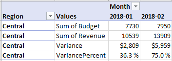
But you don’t have to leave any of those fields in the pivot table. If your manager only cares about the variance percentage, you can remove all of the other numeric fields.
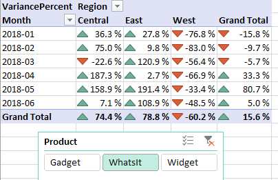
Note that the DAX in this bonus tip is barely scratching the surface of what is possible. If you want to explore Power Pivot, you need to get a copy of DAX Formulas for Power Pivot by Rob Collie and Avi Singh
DAX Formulas for PowerPivot »
Thanks to Rob Collie for teaching me this feature. Find Rob at www.PowerPivotPro.com
Watch Video
- With the Power Pivot tab, you can build relationships faster using the diagram view
- You can also insert Calculated Fields or Measures to do new calculations
- They use the DAX formula language
- They are very powerful
- Think of them as Helper Cells - they provide intermediate formulas
Video Transcript
Leran Excel from MrExcel podcast, episode 2017 – Power Pivot Formulas!
Everything in the book is going to be podcast in here, in July, August, September, go ahead and subscribe to the watch list or the playlist, top-right hand corner!
Hey, welcome back to the MrExcel netcast. Now yesterday, in episode 2016, I showed how we can just use the Data Model to take this small budget table, and this large actuals table, these three joiners, and create a Pivot table. Today I want to show you what you get if you pay the extra $2 a month to get the Office 365 Pro Plus and have Power Pivot! So here's what we're going to do, we're going to take these tables, and I'm going to add them to the data model. The budget table’s already there, I'm going to take the joiners, add that, and then back here, the Region, add that, and then the Calendar, I'll add that to the data model, and then finally, the Actuals, I'm going to add that to the data model. And I'm going to arrange these, so we have the budget on the left, the joiners in the middle.
And now, to create the relationships, this was a lot of clicks yesterday. I'm going to go from the BudTable Product, the RegTable to Region, and the Region Date down to Date. Alright, see how much faster it is to create these relationships, here in the Diagram View in the Power Pivot window. So that's one advantage, just a small advantage, I mean you can still do this with the data model, but you know, it is one small benefit. But here's the other things that we can do, once we get our report built, so we have our actuals and our budget, and remember, we use the fields from the joiner tables to build out the Pivot table. So we now have fields called Budget and Revenue, boy, it'd be really nice to show a variance, and the Power Pivot tab lets us do that.
Whether it's called a calculated item in 2013, or whether it's called a Measure in 2010 or 2016, we can create a New Measure. And this measure will be called Variance, and it's going to be equal to the Budget field minus the Actuals field, and I can even format that as currency with zero decimal places, this is cool, click OK. Alright see, so now, for each data point, we have a budget, we have an actual, and we have a Variance. What it'd be nice to take the Variance divided by the Budget to get a Variance %? So we'll insert a new measure, and this is going to be that Variance field, so the logic that I use to create the variance field is reusable, divided by the sum of Budget, and this is going to be a number, but specifically a percentage with one decimal place, alright.
So now I have 4 fields, but here's the beautiful thing, if all I want to show is the variance %, I don't need to show the Variance, the Actuals, or the Budget, I can remove those fields and the logic still works! Alright, so those are, let's call them helper formulas, that help us get to the Variance %, I only need to keep the Variance %. Everything else stays in the data model, all is understood, it's all calculated behind the scenes, and it works beautifully, and they continue to work. Even if we change the shape of the Pivot table, it keeps recalculating, it's a beautiful thing! Again, thanks to Rob Collie, and you should check out his book for the whole compendium of things you can do with these DAX formulas. And you can order Rob's book or my book online right now, use that “i” on the top-right hand corner.
Alright, episode recap: So, Excel 2013 gave us the Data Model, but you have to pay more, an extra $2 a month to get to the Power Pivot tab, the Office 365 Pro Plus will get you this. You can build relationships faster using the Diagram View, but that's really nothing new, I mean you could build relationships like I did yesterday, just using the dialog box. But it's the calculated fields or Measures that is the real benefit, it uses the DAX formula language, very powerful. They come like helper cells, they provide intermediate formulas, and you could build upon previous formulas, just really, it's where the Power in Power Pivot comes from.
Alright well hey, I want to thank you for stopping by, we'll see you next time for another netcast from MrExcel!
Download File
Download the sample file here: Podcast2017.xlsx
Title Photo: webandi / Pixabay

