Pivot Table Horizontal To Vertical

August 13, 2002 - by Bill Jelen

Fr. Mark from Kansas sent in this week's Excel question:

Excel pivot tables work best when the data is broken down into the most records possible, but this is not always the most intuitive way to load the data into Excel. For example, it is intuitive to load data like Figure 1, but the best way to analyze the data is like in Figure 2.

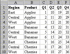
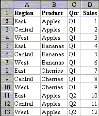
First, I will run through Excel's less-than-perfect way of dealing with multiple data fields. Second, I will demo a simple and quick macro to convert figure 1 to figure 2.

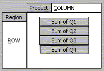
If your data is like figure 1, during PivotTable Wizard step 3 of 4, it is possible to drag all 4 quarter fields into the data area of the pivot table, as shown at right.

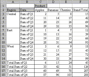
Here is the less-than-perfect result. By default, Excel has the multiple data fields going down the page. You can click on the gray "Data" button and drag it up and right to make the quarters go across the page. However, you are missing totals for each region, and the Quarter totals will always seem out of place.

So, Fr. Mark hit the nail on the head when he said that the data really needs to be in the format of Figure 2 in order to analyse it properly. Below is a macro that will quickly move data in the format of Figure 1 on Sheet1 to Sheet2 in the format of Figure 2. This macro is not general enough to work with any data set. However, it should be relatively easy to customize it to your particular situation.

Public Sub TransformData()
    ' Copyright 1999 MrExcel.com
    Sheets("Sheet2").Select
    Range("A1").CurrentRegion.Clear
    Sheets("Sheet1").Select
    Range("A1:B1").Copy Destination:=Sheets("Sheet2").Range("A1")
    Sheets("Sheet2").Select
    Range("C1").Value = "Qtr"
    Range("D1").Value = "Sales"
    Sheets("Sheet1").Select
    FinalRow = Range("A16000").End(xlUp).Row
    NextRow = 2
    LastRow = FinalRow
    ' Loop through the data columns
    For i = 3 To 6
        ThisCol = Mid("ABCDEFGHIJK", i, 1)
        ' Copy the left columns from sheet1 to sheet2
        Range("A2:B" & FinalRow).Copy Destination:= _
            Sheets("Sheet2").Range("A" & NextRow)
        ' Copy the header from ThisCol to column C
        Range(ThisCol & "1").Copy Destination:= _
            Sheets("Sheet2").Range("C" & NextRow & ":C" & LastRow)
        ' Copy the data for this quarter to column D
        Range(ThisCol & "2:" & ThisCol & FinalRow).Copy _
            Destination:=Sheets("Sheet2").Range("D" & NextRow)
        NextRow = LastRow + 1
        LastRow = NextRow + FinalRow - 2
    Next i
    Sheets("Sheet2").Select
End Sub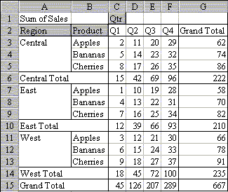

After running this macro, the data will be in the easier-to-analyze format shown in figure 2, above. Now, when you use this data for a pivot table, you have full control of the data like normal.