None of the 46,273 Built-In Styles Do What My Manager Asks For
December 15, 2022 - by Bill Jelen

Problem: My manager asks for a pivot table to be formatted with alternating stripes that are two rows high. None of the built-in styles do this.
Strategy: You can create this effect by duplicating an existing style and modifying it. Follow these steps:
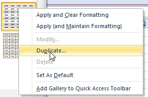
1. Find a style that is close to your manager’s request. In the PivotTable Styles gallery, right-click the style and choose Duplicate.

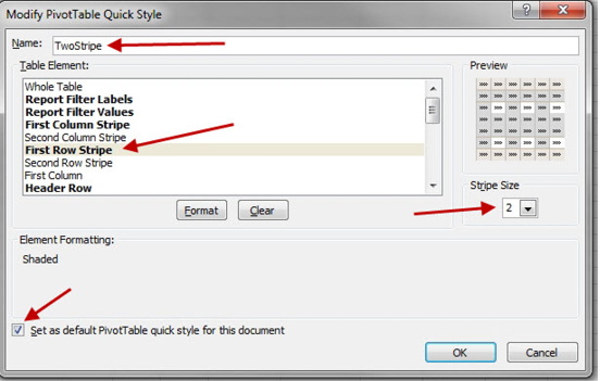
2. In the Modify PivotTable Quick Style dialog, give the style a new name. Excel initially gives the style a name by adding a 2 after the old name. Rather than PivotStyleLight 10 2, use a name like TwoStripe.
-
3. At the bottom left of the dialog, choose Set as Default PivotTable Quick Style For This Document.
4. In the Table Element list box, choose First Row Stripe. A new dropdown control appears, called Stripe Size. Open the dropdown and choose 2.

5. Repeat step 4 with Second Row Stripe.
6. Click OK to finish modifying the style. You have now created a new style, but Excel has not applied the style to your pivot table.
7. Open the PivotTable Styles gallery and find the new style at the top of the list, in the Custom section. Choose that style.
Results: A new style is available, with stripes that are two rows tall.

Additional Details: If you want all future pivot tables to use this format, right-click the style thumbnail and choose Set as Default.
Additional Details: While working in the Modify PivotTable Quick Style dialog, you can click the Format button to change the font, border, and fill.
Gotcha: The custom style is saved in the workbook. It is not available in other workbooks. Here is a workaround. Start with a blank workbook. Add a small pivot table. Format the pivot table correctly. Mark the new style as the default. Delete the data and the pivot table so you have a completely blank workbook. Save the workbook as Book.xltx as shown at Control Settings for Every New Workbook and Worksheet.
This article is an excerpt from Power Excel With MrExcel
Title photo by Agence Olloweb on Unsplash
