Manually Re-sequence the Order of Data in a Pivot Table

December 21, 2022 - by Bill Jelen

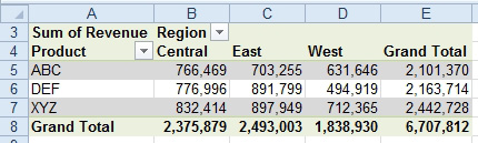
Problem: By default, a pivot table organizes data alphabetically. For the Region field, this means the data is organized with Central first, East second, and West third. My manager wants the regions to appear in the order East, Central, West. After unsuccessfully lobbying to have the Central region renamed Middle, I need to find a way to have my table sequenced with the East region first.

The region columns are in alphabetical sequence: Central, East, West. — Figure 883. Central, East, West is the alphabetical sequence.

Strategy: It is amazing that this trick works. Try it:

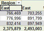
1. Select cell B4 in the pivot table.
2. In cell B4, type the word East.

Go to the Central region heading and type East. — Figure 884. Go to the Central cell and type a new heading.

3. When you press Enter, Excel senses what you are trying to do. All the data from the East region moves to Column B. Excel automatically moves the Central region heading and data to column C.

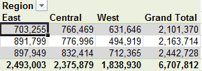
When you press Enter, the numbers from the East region move to this column. The region heading for Central and the numbers for Central move one column to the right. — Figure 885. East and Central switch! Never try this outside a pivot table.

You can easily use this trick to re-sequence the fields into any order as necessary.

Additional Details: This technique will only change the Region sequence in a single pivot table. If you would like to change the sequence in all future pivot tables, you need to create a custom list with the regions in the proper sequence. See Have the Fill Handle Fill Your List of Part Numbers. Any pivot tables created will follow the custom list sequence.

This article is an excerpt from Power Excel With MrExcel

Title photo by Toa Heftiba on Unsplash