Lookup Two Values

May 10, 2022 - by Bill Jelen

Problem: I have to lookup two values. I need to match both a company code and a cost center.

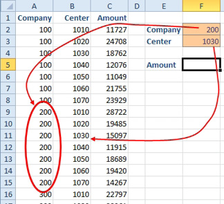
A different two-way lookup. First, you are looking for Company = 200. With Company in A and Cost Center in B, Company 100 is in rows 2 through 8. Company 200 is in row 9 through 15. Within Company 200, you are looking for Cost Center 1030. — Figure 459. Match both the Company and Center.

Strategy: There are three solutions to this problem: (a) Concatenated key, (b) OFFSET, or (c) SUMIFS. The concatenated key will only work if you are allowed to add a new column to the left of column C. The SUMIFS will only work if the value to be returned is numeric. The OFFSET will only work if all of the company codes are sorted together as shown above.

With a concatenated key, you will insert a new column before the Amounts in column C. You want to join column A, a unique separator, and column B. For example, =A2&”-”&B2 would produce a key of 100-1010.

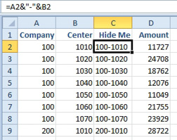
Solution 1 is a concatenated key in column C. The heading is Hide Me. Column C contains company dash center. — Figure 460. Build a concatenated key in your data.

The separator text is optional. In real life, you might have two company/center combinations that would look the same once joined. Using a dash in between will prevent this ambiguity.

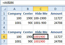
The dash in Hide Me is important. WIthout the dash, you can imagine Company 100 Center 1900 giving you 1001900 which is the same as Company 1001 and Center 900. — Figure 461. Using a dash prevents the identical key fields in red.

Once you have the concatenated key in the lookup table, you can join the key fields on-the-fly in your VLOOKUP formula:

=VLOOKUP(G2&”-”&G3,$C$2:$D$22,2,FALSE)

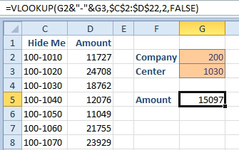
The VLOOKUP becomes =VLOOKUP(G2&"-"&G3 into the HideMe column. — Figure 462. Join the two key fields as the first argument of VLOOKUP.

As mentioned earlier in this topic, this method only works if you are able to add the concatenated key to your data. It is fine to hide column C so no one see it, but you have to have the field there.

Alternate Strategy: If the value that you are trying to return is numeric, you can use DSUM or SUMIFS. For details, see Calculate Based on Multiple Conditions.

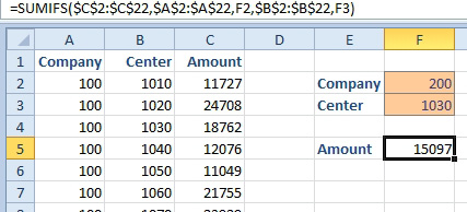
Another solution, only if the value being returned is numeric, is a SUMIFS formula. Total the values where Company=100 and Cost Center = 1030. — Figure 463. The new SUMIFS would solve the problem.

Alternate Strategy: Use the OFFSET function. Purists will argue that OFFSET is a volatile function and therefore slows down your calculation times. However, OFFSET will often solve problems where you need to reference a range that is moving or resizing.

OFFSET is used to point to a range. The location and size of the range is calculated as the formula is being calculated.

OFFSET allows five arguments. At least one of the four final arguments should be a formula that is calculated on the fly. When OFFSET is set up to return a range of cells, you will find yourself using OFFSET inside of another function such as SUM, or in this case, inside of VLOOKUP.

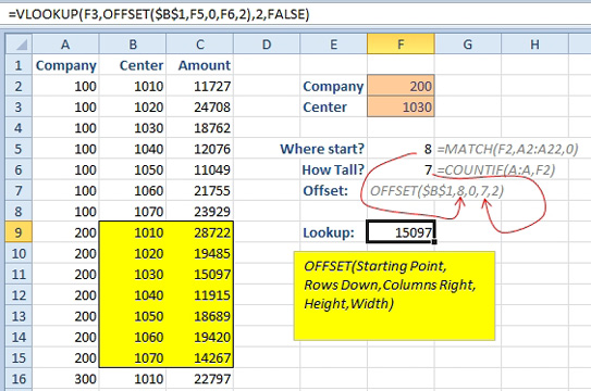
The syntax is =OFFSET(Reference,Rows Down from There, Columns Right from There, Rows Tall, Columns Tall). For example, you could start with a reference of B1, move down N rows, move right 0 rows, make the range be 7 rows tall and 2 columns wide.

In the next figure, a MATCH function in F5 figures out where the lookup table for this company begins. The COUNTIF in F6 figures out how tall the lookup table should be. Both of these numbers will feed into an OFFSET function that is shown for illustration in F7. The actual formula is found in F9, where the OFFSET is used to describe the lookup table in the VLOOKUP formula.

A third solution is volatile. Use MATCH to figure out that company 200 starts in row 8. Use COUNTIF to figure out that Company 200 is 7 rows tall. Then, the lookup table becomes OFFSET($B$1,8,0,7,2). — Figure 464. OFFSET is slow, but versatile.

This article is an excerpt from Power Excel With MrExcel

Title photo by AbsolutVision on Unsplash