
Limit a Pivot Report to Show Just the Top 5 Customers
December 29, 2022 - by Bill Jelen

Problem: Many times my customer reports have hundreds of customers. If I’m preparing a report for the senior vice president of sales, he may not care about the 400 customers who bought spare batteries this month. He wants to see only the top 10 or 20 or 5 customers each month.
Strategy: You can accommodate this vice president by using the Top 10 Filter feature that is available in pivot tables. Follow these steps:
1. Build a pivot table with Customers in the row area.
2. Open the dropdown at the top of the customer dropdown. Choose Value Filters and then Top 10.
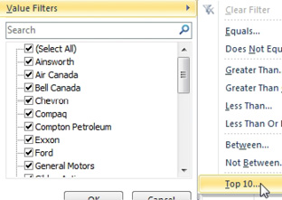
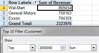
Excel displays the Top 10 Filter (Customer) dialog. By default, the dialog wants to show the top 10 items based on Sum of Revenue. Although it is called the “Top 10” feature, it is far more flexible than that. The first dropdown offers to filter to the top or bottom customers. You can use the spin button to change 10 to any other number. The third field offers Items, Percent, and Sum.
3. Change 10 to 5.
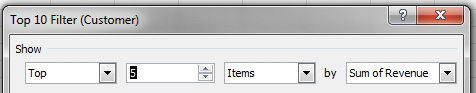
4. Click OK.
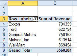
Results: The report will be filtered to show just the top five customers. Note that a Filter icon appears in cell A3 to indicate that you are not seeing all customers. You can hover over this icon to see a list of the filters applied
Gotcha: If there is a tie for fifth place, the list may contain more than five customers. If you filter the pivot table to an obscure product purchased by only a few customers, you might have a hundred-way tie at $0 for fifth place.
Additional Details: Another common request might be to show enough customers to represent 80% of the total.
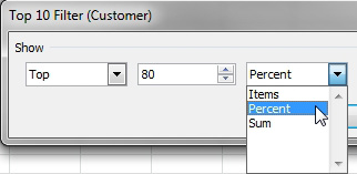
Or, you can ask for enough customers so the sum is $2,000,000. Excel will include the largest customers until the total is over $2,000,000.
Gotcha: The total on each report includes only the customers shown in that report. My VP of Sales wants the other customers grouped into one line called Other. See the next topic for an alternate strategy.
Additional Details: To clear a filter, you use the dropdown at the top of that column and select Clear Filters from Customer..
This article is an excerpt from Power Excel With MrExcel
Title photo by Joshua Hoehne on Unsplash