Inserting Alternating Rows
May 24, 2018 - by Bill Jelen

Today's question from the Atlanta Power Excel seminar.
I have data formatted with every other row in grey. When I insert two new rows in the middle of the data, both of the new rows end up grey instead of following the pattern.
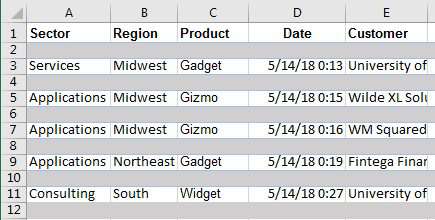
Take a look at the workbook in the image below. The even numbered rows have a grey fill.
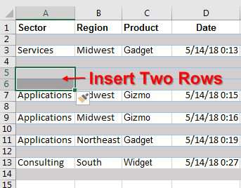
When you select A5:A6 and Insert Rows, you get two new blank rows. But both rows are grey.
I have a solution to this, but it requires a trip back to 3rd grade math.
In 2nd or 3rd grade, when you were first learning division, you might remember this:
- 4 Goes In to 9: 2 with a Remainder of 1 or 2R1
- 5 Goes in to 17: 3 with a Remainder of 2 or 3R2
In elementary school, you called this a remainder. I find a lot of people remember this.
But later, in high school, when most of us had stopped paying attention to Math, they introduced the concept called Modulo.
17 Modulo 5 is 2.
Modulo is derived from the Latin word Modulus.
In English, this says: "Divide 5 in to 17 and the remainder is 2"
In Excel, you can calculate a Modulo using =MOD(17,5). Here are some MOD results:

This article is supposed to be about shading rows in grey. Why all the math theory? Because MOD solves this problem!
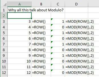
Check out column A below. The =ROW() function tells you what row you are in.
And column C divides the number 2 in to the Row number and gives the remainder. For even rows, the remainder is 0. For odd rows, the remainder is 1.
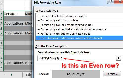
Set up conditional formatting to check to see if the MOD(ROW(),2)=0:
- Select all of the cells in your data.
- Home, Conditional Formatting, New Rule.
- Use a Formula to Determine Which Cells to Format.
-
The formula is
=MOD(ROW(),2)=0 - Click Format... and apply a grey fill.
- Click OK.
Every other row is formatted in grey. But - the beautiful advantage - as you insert new rows, they keep the alternating grey/white color. (Check out the video below to see this in action.)
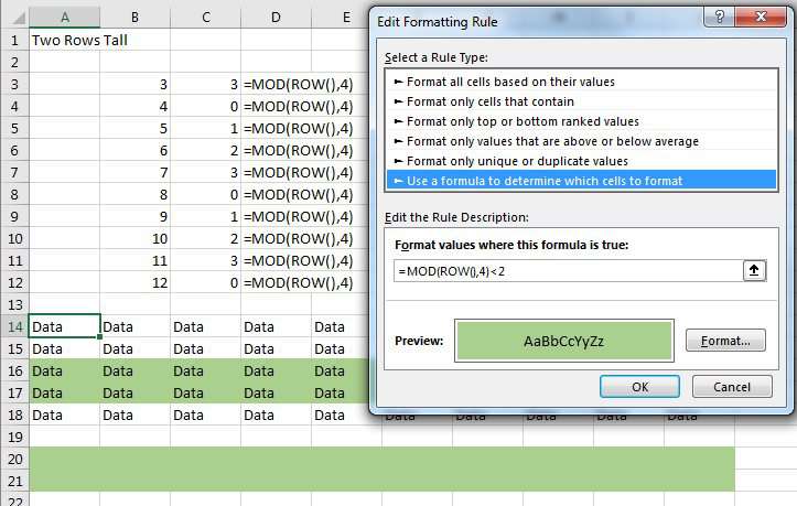
You can extend this concept. Say you want two rows of green followed by two rows of white. Calculate =MOD(ROW(),4). The four possible answers are 0, 1, 2, and 3. Set up a rule to test if the result is <2 and format those rows in green.
Watch Video
Video Transcript
Learn Excel from MrExcel Podcast Episode 2209: Inserting Alternating Rows.
Hey, welcome back to the MrExcel netcast, I'm Bill Jelen. This one's a classic-- I was down in Atlanta and someone described that they had a spreadsheet like this. Now, hey, I don't want to hear that you shouldn't keep your spreadsheet like this; they had a spreadsheet like this, and they said, "Here's our problem. We have 2 physical rows for every data, and whether we should do that or not, when I insert 2 rows, Alt+I+R and insert 2 rows, all 3 rows freaking become gray!" I said, "Ah, yeah, I've got a solution for this."
But, before we get to that solution, we have to go back to, like, third grade/second grade, when you're first learning how to divide. Remember this? 4 goes into 9: 9/4, and the answer would be 2 with a remainder of 1. 4 goes into 9 2 times; 4x2=8; there's 1 leftover. So we would write 2R1. 5 goes into 17 3 times with a remainder of 2; 3R2. You remember remainders, right? That's because we were all paying attention in third grade. This stuff was hard back in third grade. In high school, no one was paying attention to math anymore-- we were paying attention to the pretty girl sitting in front of us-- and so you don't remember when your math teacher taught you about something called Modulo.
Modulo is just like remainders. 17 Modulo 5 is 2 because 2 is the remainder when you divide 5 in to 17. You get 3 with a remainder of 2. So, if we asked for =MOD(17,5), the answer's going to be 2. MOD stands for Modulo, which is really just some fancy name for remainder. That's the remainder. Alright, why all this talk about Modulo?
So, I'm going to use a function here =ROW, and =ROW just tells me what row it's in (3, 4, 5, 6, 7, 8, 9, 10, 11, 12...) and then I'm going to take the =MOD of that row, divided by 2. Alright, so 2 goes in to 3 1 time with a remainder of 1. 2 goes into 4 twice with a remainder of 0. This formula over here is going to give me only 2 possible answers: either 0 or 1, 0 or 1. And the beautiful thing is, when I insert a new row, those zeroes or ones-- they're going to adjust. So, basically, a 1 is going to give me every odd row, and a 0 is going to give me every even row. It looks like here I want to highlight the even rows. So, I'm just going to choose all this data, and I'm going to go into Conditional Formatting. Home; Conditional Formatting; New Rule; Format Cell; Use a formula to determine which cells to format; and I'm going to ask =MOD(ROW(),2)=0 and, if it is, then what I want to do is I want to format that with a gray background-- fill of gray; click OK; click OK; and bam-- every other row is gray, just like we started out with in Atlanta before I inserted those two rows and screwed everything up. But the beautiful thing about this is when I decide that I need more data, and I insert 2 rows-- Alt+I+R-- the rows are formatted in white and gray, like I wanted. And I could even insert 2 rows right here-- Alt+I+R-- and it still continues to format in white and gray like I wanted. Modulo-- it's a remainder.
Alright, now that we've got that one down, let's do 2 rows tall. Back in the day, when we printed our Green Bar reports, our Green Bar reports-- they weren't 1 row, 1 row, 1 row, it was 2 rows, 2 rows, or maybe even 4 rows, 4 rows. Alright? So, if I want to do 2 rows tall-- here's our =ROW function, and then I take the =MOD of that row number and divide it by 4, and we'll drag both of these down and see what we get. We're going to get 4 possible answers now-- 0, 1, 2, or 3. So, the whole question is, is the =MOD(ROW,4)= 0 or 1, 2 or 3? Your choice. Choose all this data down here; Alt+O+D for Conditional Formatting; New Rule; "Use a formula"; then we say =MOD(ROW(),4)=<2 (so, the choices are 0, 1, 2, 3. I want to highlight every other one, so =<2; that means is it 0 or 1?); and if it is, I'm going to choose the same green that we had back in the IBM printers back in the 1980s (yes, I'm that old); click OK; click OK; and BAM! we now have the every row being 2 tall, then 2 tall, then 2 tall, 2 tall, and again, it works beautifully if I insert a whole bunch of more rows, I keep that green bar format all the way down.
I love when I get a great Excel question that I know the answer, and the answer involves some sort of weird, geeky math because now it's geeky Excel, and geeky math. The word Modulo-- I don't know if it's Latin or Greek, or who knows what it is, but it solves that problem.
MrExcel LIVe: The 54 Greatest Excel Tips of All Time. Click that "I" up there in the top righthand corner to read more about that book.
Wrap-up of this episode from the Gulf South Council at the IMA Seminar in Atlanta-- hey, I have data formatted with every other row of gray; When I insert two rows, both rows are gray. I have a great solution with Conditional Formatting but requires third grade math. Divide the row number by 2. What's the remainder? It's either going to be 0 or 1. So, set up Conditional Formatting, check to see if =MOD(ROW(),2)=1 and if it is, then fill that row with gray. It works awesomely.
Feel free to download the workbook -- the URL's down there in the Youtube description-- and set up a =MOD function to highlight 3 rows in orange and 1 row in teal, and that's right. You can create hideous looking workbooks, too, just using the =MOD function. I want to thank you for stopping by. I'll see you next time for another netcast from MrExcel.
Download Excel File
To download the excel file: inserting-alternating-rows.xlsx
Excel Thought Of the Day
I've asked my Excel Master friends for their advice about Excel. Today's thought to ponder:
"Two spreadsheets are better than none."
Title Photo: Samuel Zeller on Unsplash
