Help Your Kids with Their Math

March 11, 2022 - by Bill Jelen

Problem: My kids have math homework, and I want to check their answers. They are doing least common multiples, greatest common denominators, Roman numerals, and factorials.

Strategy: You can easily solve problems involving least common multiples, greatest common denominators, roman numerals, and factorials using Excel.

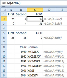
Least Common Multiples: When you have to add fractions that have different denominators, one of the first steps is to find the least common multiple of the two denominators. The math homework asks your kids to add 3/26 + 3/4. You want to figure out the least common multiple of 26 and 4, so enter 26 in one cell and 4 in another cell. The formula to find the least common multiple is =LCM(A2:B2). The answer is 52. You can now have your kids change 3/26 to 6/52 and 3/4 to 39/52. Expressing the problem as 39/52 + 6/52 makes it easy to see that the answer is 45/52.

Greatest Common Denominators: This time, the problem is 2/9 + 2/4. The LCM of 9 and 4 is 36 as shown in row 3 above. You can change 2/9 to 8/36 and 2/4 to 18/36. The problem then becomes 8/36 + 18/36. The answer is 26/36. However, can the fraction 26/36 be further reduced? You need to find the greatest common denominator of 26 and 36. To do so, you use the GCD function =GCD(A6:B6). Because the answer is greater than 1, your 26/36 answer can be reduced by dividing both the numerator and denominator by 2; 26/36 is the same as 13/18.

Excel has functions to calculate Least Common Multiple and Greatest Common Denominator. — Figure 371. Middle school math.

Roman Numerals: Your kids are supposed to use Roman numerals. To do this, you can use the ROMAN function as shown in rows 9:14.

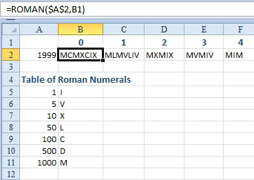
The ROMAN function will work with numbers from 1 to 3,999. If you omit an optional second argument, you will get classic Roman numerals, as shown above.

Calculating Roman numerals is fairly obscure. Other than middle school students and Latin teachers, who has to do this? The NFL commissioner needs to calculate future Super Bowl numbers. The people who do movie credits need to figure out the information to use in the copyright line. Excel wasn’t invented when Foreigner IV was released and I somehow doubt that that Holy See fires up Excel when naming the next pope.

If you remember the basics of Roman Numerals, I is 1, V is 5. To show 7, you would use VII. But, to show 4, you would use IV. Since the I occurs before the V, it represents 1 subtracted from 5. Modern convention says that you can represent 4 with IV and 9 with IX, but you can not use IL for 49. The optional second argument of the ROMAN function allows you to break the rules more and more.

The ROMAN of 1999 is five formats is shown. With a second argument of 0, you get the normal result of MCMXCIX. Each of the other numbers 1 to 4 results in shorter results: MLMVLIX, MXMIX, MVMIV, MIM — Figure 372. Excel offers more concise Roman numerals.

Starting in Excel 2013, you can convert Roman numerals back to regular numbers using the =ARABIC() function. This isn’t a function that Microsoft wanted to add to Excel. But, since they are trying to remain compliant with the Open Document Spreadsheet standard, it was added to Excel 2013.

The =ARABIC("MMXIV") returns 2014. — Figure 373. Convert from Roman back to Arabic.

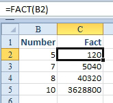
Factorials: The last obscure function you need to help with the math homework is the factorial function, FACT. A factorial is a number multiplied by every integer between itself and 1. To write 5 factorial, you use the number followed by an exclamation point. So, for example, 5! is 5 x 4 x 3 x 2 x 1, or 120. Use =FACT(5) to calculate 5!.

Calculating 5 Factorial with =FACT(5). This is 5*4*3*2*1 and is 120. — Figure 374. The factorial of 5 is 5 x 4 x 3 x 2 x 1, or 120.

This article is an excerpt from Power Excel With MrExcel

Title photo by David Libeert on Unsplash