
Grouping 1 Pivot Table Groups Them All
January 17, 2023 - by Bill Jelen

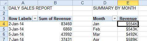
Problem: I am building two pivot tables. One will show daily sales detail. The other will summarize by month. I arranged the pivot tables side by side. I use the Group feature to group the second pivot table by month.
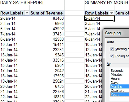
Unfortunately, this groups both pivot tables by month.
Strategy: One solution is to group by Days, Months, and Years. You can then use different fields in the two pivot tables. However, the point of this topic is how to create two pivot tables that do not share the same pivot table cache.
When you create a pivot table, the data from your worksheet is loaded into memory to a special area called the pivot table cache. A pivot table is fast because it is calculated from the cache in memory.
Way back in Excel 2003, Excel would ask you if you wanted all of your pivot tables to share the same pivot table cache. This would save memory...each pivot table cache increases the size of the workbook by the amount of data in the data set. But, sharing a cache causes problems like the one here; when you group fields or calculate fields, those changes happen in all of the pivot tables.
In Excel today, any pivot table created using Insert, PivotTable automatically shares the cache. Microsoft doesn’t even ask you.
However, you can force Microsoft to ask if you want to share the cache by using the old pivot table wizard. Follow these steps
1. Create the first pivot table as normal.
2. To create the second pivot table, select one cell in your original data set.
3. Press Alt+D followed by P. This was the Excel 2003 keyboard shortcut for Data, PivotTable. Excel will display step 1 of the old pivot table wizard.
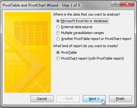
4. Click Next in step 1.
5. Make sure your data range is correct in step 2.
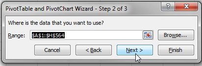
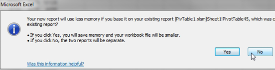
6. Click Next. Between Step 2 and Step 3, Excel will display a lengthy message that encourages you to have this pivot table share the cache with the other pivot table in order to conserve memory. You want to click No to this dialog.
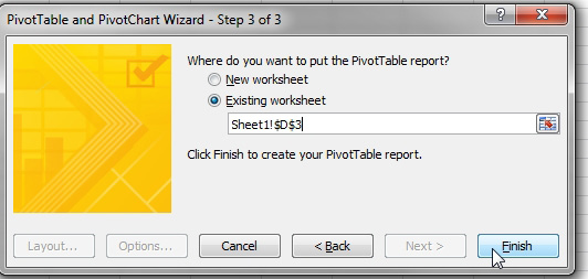
7. In Step 3 of the wizard, choose the location for your pivot table. Click Finish.
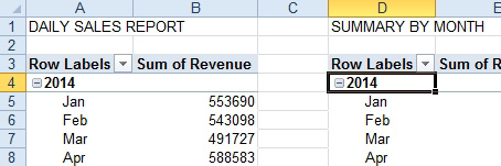
You can group the second pivot table and it will not affect the first pivot table.
This article is an excerpt from Power Excel With MrExcel
Title photo by Ashim D’Silva on Unsplash