GetPivotData
August 28, 2017 - by Bill Jelen

Do you hate Excel's GETPIVOTDATA function? Why does it appear? How can you prevent it? Is there a good use for GETPIVOTDATA?
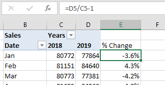
Most people first encounter GETPIVOTDATA when they try to build a formula outside a pivot table that uses numbers in the pivot table. For example, this variance percentage won’t copy down to the other months due to Excel inserting GETPIVOTDATA functions.

Excel inserts GETPIVOTDATA any time you use the mouse or arrow keys to point to a cell inside the pivot table while building a formula outside the pivot table.
By the way, if you don’t want the GETPIVOTDATA function to appear, simply type a formula such as =D5/C5-1 without using the mouse or arrow keys to point to cells. That formula copies without any problems.
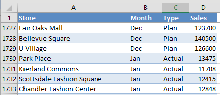
Here is a data set that contains one plan number per month per store. There are also actual sales per month per store for the months that are complete. Your goal is to build a report that shows actuals for the completed months and plan for the future months.
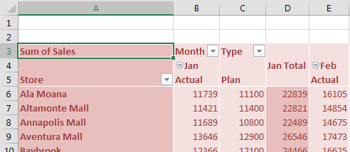
Build a pivot table with Store in ROWS. Put Month and Type in the COLUMNS. You get the report shown below, with January Actual, January Plan, and the completely nonsensical January Actual+Plan.
If you select a month cell and go to Field Settings, you can change subtotals to None.
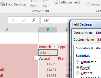
This removes the useless Actual+Plan. But you still have to get rid of the plan columns for January through April. There is no good way to do this inside of the pivot table.
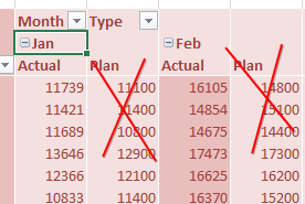
So, your monthly workflow becomes:
- Add the actuals for the new month to the data set.
- Build a new pivot table from scratch.
- Copy the pivot table and paste as values so it is not a pivot table anymore.
- Delete the columns that you don’t need.
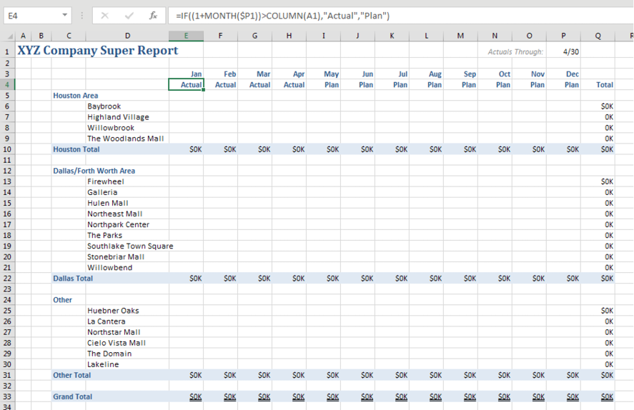
There is a better way to go. The following very small figure shows a new Excel worksheet added to the workbook. This is all just straight Excel, no pivot tables. The only bit of magic is an IF function in row 4 that toggles from Actual to Plan based on the date in cell P1.
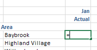
The very first cell that needs to be filled in is January, Actuals for Baybrook. Click in that cell and type an equal sign. Using the mouse, navigate back to the pivot table. Find the cell for January Actuals for Baybrook. Click on that cell and press Enter. As usual, Excel builds one of those annoying GETPIVOTDATA functions that cannot be copied.
But today, let’s study the syntax of GETPIVOTDATA.
The first argument below is the numeric field "Sales". The second argument is the cell where the pivot table resides. The remaining pairs of arguments are field name and value. Do you see what the auto-generated formula did? It hard-coded "Baybrook" as the name of the store. That is why you cannot copy these auto-generated GETPIVOTDATA formulas. They actually hard-code names into formulas. Even though you can't copy these formulas, you can edit them. In this case, it would be better if you edited the formula to point to cell $D6.

Here is the formula after you edit it. Gone are "Baybrook", "Jan", and "Actual". Instead, you are pointing to $D6, E$3, E$4.
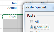
Copy this formula and then choose Paste Special, Formulas in all of the other numeric cells.

Now here's your annual workflow:
- Build an ugly pivot table that no one will ever see.
- Set up the report worksheet.
Each month, you have to:
- Paste new actuals below the data.
- Refresh the ugly pivot table.
-
Change cell P1 on the report sheet to reflect the new month. All the numbers update.
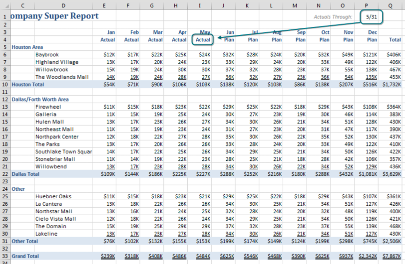
Change Cell P1
You have to admit that using a plain report that pulls numbers from a pivot table gives you the best of both worlds. You are free to format the report in ways that you cannot format a pivot table. Blank rows are fine. You can have currency symbols on the first and last rows but not in between. You get double-underlines under the grand totals, too.
Thanks to @iTrainerMX for suggesting this feature.
Watch Video
- GetPivotData happens when a formula points inside of a pivot table
- While the initial formula is correct, you can not copy the formula
- Most people hate getpivotdata and want to prevent it
- Method 1: Build a formula without the mouse or arrow keys
- Method 2: Turn off GetPivotData permanently using the dropdown next to options
- But there is a use for GetPivotData
- You manager wants a report with Actuals for past months and budget for future
- The normal workflow would have you create a pivot table, convert to values, delete columns
- Removing Subtotals to prevent January Actual+Plan using Field Settings
- Instead, create a pivot table with "too much" data
- Use a nicely formatted report worksheet
=IF((1+MONTH($P1))>COLUMN(A1),"Actual","Plan")- From the first data cell on the worksheet, build a formula with the mouse
- Allow GetPivotData to happen
- Examine the syntax of GetPivotData (field to return, pivot location, pairs)
- Change the hard-coded value to point to a cell
- Pressing F4 three times locks only the column
- Pressing F4 two times locks only the row
- Paste Special Formulas
- Workflow next month: Add data, refresh pivot table, change through date
- Ultra careful to watch out for new stores
Transcript of the Video
Learn Excel from MrExcel podcast, episode 2013 - GetPivotData May Not Be Entirely Evil!
I'll be podcasting this entire book, click that “i” on the top-right hand corner to subscribe.
Alright, back in episode 1998 I talked briefly about this GetPivotData problem. If we calculate a % variance and we're outside of the Pivot table pointing inside, and I use the mouse or the arrow key, so 2019/2018-1. This answer that we're going to get here is correct for January, but when we double click to copy that down, the formula does not copy, we get the January answer all the way down. And when we look at it, we're getting GetPivotData, I didn't type GetPivotData, I just pointed to those cells, and this started happening back in Excel 2002 without any warning whatsoever. And at that point I said that the way to avoid this is to type up the formula C5/B5-1, and you'll get a formula that you can copy. Or if you just hate GetPivotData, if it's “completely evil”, go to the Analyze tab, don't open the Options button by the way. Go back to the Pivot table, go to the Analyze tab, open the dropdown next to Options, uncheck this box, it's a global setting. Once you turn it off, it'll be off forever, alright.
Most of the time the questions I get are “How do I turn GetPivotData off?” but every once in a while I will get someone who loves GetPivotData. And I was having lunch with Rob Collie when he was still at Microsoft, and he said “Well, our internal customers love GetPivotData.” I said “What? No, everyone hates GetPivotData!” Rob says “You're right, outside of Microsoft, absolutely, they hate GetPivotData.” I'm talking about the accountants inside of Microsoft, and later I met one who now works for the Excel team, Carlos, and Carlos was one of the accountants who use this method.
Alright, so here's what we have to do. We have our report, a data set here that for every month we have the plan for each store, and then at the bottom we are accumulating actuals. Alright, so we have actuals for January through December, but only have actuals for a few months, the months that have gone past. And what our manager wants us to do is build a report with stores down the left-hand side, only the Texas stores, of course, to make life more difficult. And then going across we have months, and if we have an actual for that month, we show the actual, so January actual, February actual, March actual, April actual. But then for the months where we don't have actuals we switch over and show the budget, so budget out through December, and then a total totaling everything, alright. Well, when you try and create this Pivot table, yeah, it doesn't work.
So insert PivotTable, New Worksheet, you put Store down the left-hand, side that's beautiful, put Months across the top, put Type across the top, put Sales here, alright. So here's what we get that we have to start to work with, so we have January actual, January plan, and then the completely useless January actual plus plan. No one will ever use this, but I can get rid of these gray columns, that's easy enough, some here to this cell, go to Field Settings, and change the Subtotals to None. But there's absolutely no way for me to remove the January plan that won't also remove the April May June July plan, alright, there's no way to get rid of this. So at this point every month, I'm stuck selecting the entire Pivot table, going to Copy, and then Paste, Paste Values. It's not a Pivot table anymore, and then I start manually deleting the columns that don't appear in the report.
Alright, that's the normal method, but the accountants at Microsoft have added an extra step in January, it takes 15 minutes, and this that step allows this Pivot table to live forever, right? I call this the world's ugliest Pivot table, and the accountants at Microsoft accept that this is the world's ugliest Pivot table, but no one will ever see this report except for them. What they do, is they come here to a new sheet, and build the report that their manager wants. Alright, so here's the stores down the left-hand side, I even grouped it into Houston, Dallas and Other, it's a nicely formatted report. I've highlighted the totals, you'll see that when we get some numbers in, there's currency on the first row, but not these subsequent rows, blank rows. Ooh, blank rows in the Pivot table. And one tiny bit of logic up here, where I can put the through date in cell P1, and then I have a formula here that analyzes that IF the month of the through date is > this column, and then put the word Actual, otherwise put the word Plan, alright. So all I have to do has change this through date, and then the word Actual flip over to plan, Alright.
Now, here's what we do, we're going to allow ourselves to be GetPivotData’d, right? I'm not sure that that's a verb, but we're going to allow Microsoft to GetPivotData. So I start building a formula with an =, I grab the mouse, and I'm going to go look for January actual Baybrook! So I go back into the world's ugliest Pivot table, I find Baybrook, I find January, I find actual, and I click Enter, and let them do it to me, alright, there we go, we now have a GetPivotData formula. I remember the day that I did this, it was like, you know, after Rob explained to me what they were doing, and I went back and tried it. Now all of a sudden, all my life, I've been getting rid of GetPivotData, I've never actually embraced GetPivotData. So what it is, is the first item is what we're looking for, there's a field called Sales, this is where the Pivot table starts, and it can be any cell in the Pivot table, they use the top-left hand.
Alright, this is a field name “Store”, and then they've hardcoded ”Baybrook”, this is a field name “Month”, they've hardcoded “January”, this is a field name “Type”, and they've hardcoded “Actual”. THAT's why you can't copy it, because they've hardcoded the values. But the accountants at Microsoft, Carlos and his co-workers realize “Whoa, wait a second, we have the word Baybrook here, we have January here, we have Actual here. We just need to change this formula to point to the actual cells in the report instead of being hardcoded.” Alright, so they call this parameterizing the GetPivotData.
Remove the word Baybrook, come over here and click on cell D6. Now, I need to lock this down to the column, alright, so I press the F4 key 3 times, get a single $ before the D, alright. For the month of January I remove the hardcoded January, I click on the cell E3, I'll press F4 twice to lock it down to the row, E$3. Type Actual, remove the word Actual, click on E4, again F4 twice, alright, and I get a formula that now pulls that data back. I'm going to copy that, and then Paste Special, choose Formats, Alt E S F, see the F is underlined there, E S F Enter, and then now that, I've done that I'll just repeat with F4, F4 is a redo, and F4. Alright, so now we have a nice-looking report, it has blanks, it has formatting, it has the single accounting underline under each section, at the very bottom it has the double accounting underline.
Right, you never get this stuff in a Pivot table, that's impossible, but this report is driven from the Pivot table. So then what we do when we get the May actuals, come back here, paste them in, go refresh the world's ugliest Pivot table, and then here on the report just change the through date from 4/30 to 5/31. And what that does is that causes this formula switch over from the word Plan to Actual, which goes and pulls the actuals from the report, instead of the plan, alright. Now, here's the thing that- this is a great, right? I can see where I would do this a lot if I still, you know, worked in accounting.
The thing that you have to be really careful about is if they build a new store, you have to know to add it in manually, right, the data is going to show up in the Pivot table, but you would add it manually. Now this one is a subset of all the stores, if it was reporting all the stores, I would probably out here, outside of the print range, have something that pulled the grand total from the Pivot table. And then I would know, if this total doesn't match the grand total from the Pivot table, that something's wrong, and have an IF function down here Saying “Hey there's, you know, new data that's been added, be very careful.” They have some sort of a mechanism to detect that new data is there. But I get it, it's a cool use. So, while most of the time GetPivotData just drives us crazy, there can actually be a use for it. Alright, so that's tip #21 out of 40 in the book, buy the book right now, order online, click that “i” on the top-right hand corner.
Long, long recap today, alright: GetPivotData happens when a formula points inside of a Pivot table, a formula outside the Pivot table points inside. While the initial formula is correct, it won't copy. Most people hate GetPivotData and want to prevent it. So you can build a formula without the mouse or the arrow keys, just type the formula, or turn off GetPivotData permanently, ah, but there's a use, alright. So we have to build a report with actuals for past month, budget for future. Normal workflow, create a Pivot table, convert to values, Delete columns. There is a way to remove the subtotals by using Field Settings, getting rid of that January actual plus plan. Instead we're just going to create the world's ugliest Pivot table with too much data.
Build a nicely formatted, just plain old report worksheet with maybe a little bit of logic to change the word Actual to Plan. And then from the first report cell, the first place where numbers are going to be in that report, type an =, go point to the Pivot table and allow GetPivotData to happen. We examine the syntax of GetPivotData, so it's the field to return, Sales, where the Pivot table lives, and then pairs of criteria, the field name and the value. We're going to remove the hardcoded value and point to a cell, pressing F4 3 times locks only the column, pressing F4 2 times locks only the row, copy that formula, Paste Special Formulas. I threw in an extra tip there that F4 is a redo, so I only had to go to the Paste Special dialog once, and then for the next Paste Special Formulas just used F4. Next month add the data, refresh the Pivot table, change the through date. Make sure they didn't build any new stores, you know, have some sort of a mechanism, either manual, or a check formula, check it out. Thanks to iTrainerMX on Twitter, who suggested GetPivotData, also Carlos and Rob from Microsoft, Rob now from Power Pivot Pro. Carlos for using this, and Rob for telling me that Carlos was using it, I met Carlos later, and he confirmed yes, he was one of the accountants who used this all the time at Microsoft, alright, there you go.
Well hey, I want to thank you for stopping by, we’ll see you next time for another netcast from MrExcel!
Download File
Download the sample file here: Podcast2013.xlsx
Title Photo: Hans / pixabay
