Get Excel Data Into Power Pivot

March 09, 2023 - by Bill Jelen

Problem: How do I get my Excel data into Power Pivot?

Convert your Excel data to a table and then link the table to Power Pivot.

First, convert your dataset to a table by selecting one cell and pressing Ctrl+T. Excel will ask you to confirm that your data has headers. Click OK. On the Table Tools Design tab, enter a new name for the table on the left side of the ribbon. This name will carry through to Power Pivot and be used in formulas later, so keep it short and easy to spell.

On the Power Pivot tab, choose Add to Data Model in Excel 2013 or Create Linked Table in Excel 2010.

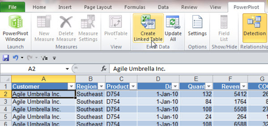
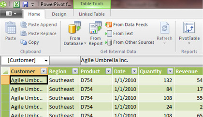
On the PowerPivot tab of the Ribbon, choose Create Linked Table — Figure 1053. Define your data as a table, you can simply link to the table.

After a moment, you will see your data in the green grid of the Power Pivot window.

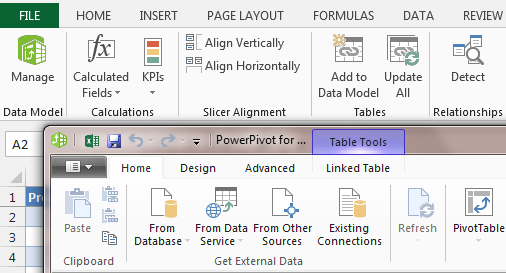
The same data from the Excel table is shown in the Linked Table tab of the Power Pivot window. — Figure 1054. The linked table appears in Power Pivot.

There is a Power Pivot tab in the Excel ribbon. In Excel 2013, click the Manage button to open Power Pivot. In Excel 2010, click the Power Pivot Window icon to open Power Pivot.

The Excel ribbon offers a Manage icon (both on the Data tab and the Power Pivot tab). Click Manage and you launch a Power Pivot window with a new Ribbon: Home, Design, Advanced, Linked Table. — Figure 1055. Although Excel offers a Power Pivot ribbon, most commands are inside of Power Pivot.

This article is an excerpt from Power Excel With MrExcel

Title photo by Towfiqu barbhuiya on Unsplash