
Find Differences In Two Lists
October 31, 2022 - by Bill Jelen

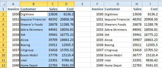
Problem: I have two lists that should be identical. I need to highlight any cells that are different.
Strategy: Use the Go To Special dialog’s Row Differences.
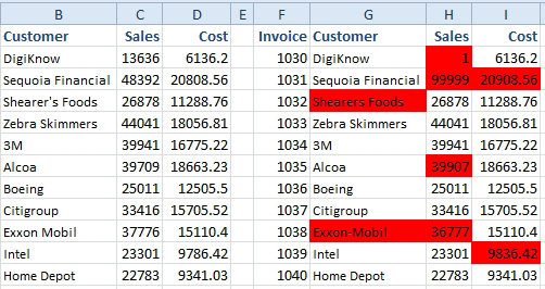
1. Select B2:D12.
2. Hold down the Ctrl key while selecting G2:I12.
-
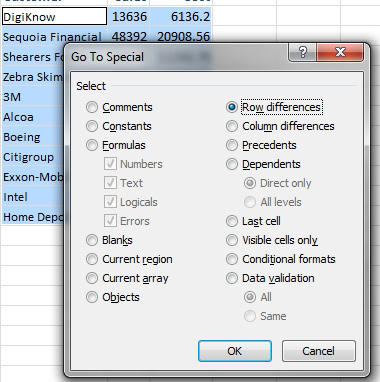
3. Choose Home, Find and Select, Go To Special.
4. In the Go To Special dialog, choose Row Differences. Click OK.
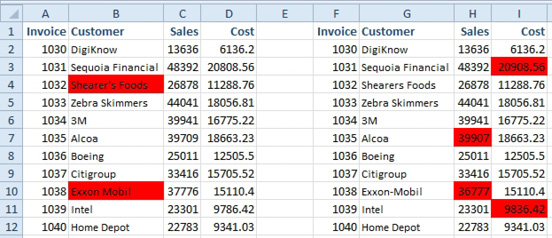
Gotcha: Highlight row differences can only compare one column to another column. Initially, it will only compare column B to column G and highlight what changed. If you then press the F4 key once for each additional column, the program will redo the compare for the next column and then the next column.
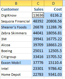
After step 4, you will have this:
5. Press the F4 key to compare column C to column H.
6. Press the F4 key to compare column D to column I.
7. Open the Paint Bucket icon on the Home tab and choose a fill color.
Result: All of the changed cells will be highlighted, in one list or the other.
Alternate Strategy: You can use the Formula method of conditional formatting to highlight differences. Follow these steps:
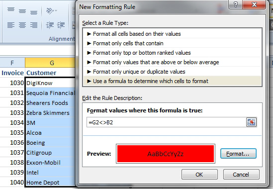
1. Select G2:I12.
2. Type Alt+O followed by D. (That is O the letter).
3. Click New Rule.
4. Choose Use a Formula to Determine Which Cells to Format.
5. Type a formula of
=G2<>B2.6. Click the Format… button.
7. Click the Fill tab.
8. Choose a red format.
9. Click OK. Click OK.
The changed cells on the right are highlighted.
This article is an excerpt from Power Excel With MrExcel
Title photo by Pierre Bamin on Unsplash