Fast Multi-Column VLOOKUP

April 21, 2022 - by Bill Jelen

Problem: I have to do twelve columns of VLOOKUP. The lookup table is large. The data set is even larger. It is taking forever to calculate.

VLOOKUP is an expensive function. It takes a lot of time to find the exact match in the lookup table. Worse, consider one row of your table. Excel might have to search through a 200-row table to locate the SKU when looking up the January value. When Excel goes to look up the February value, it must begin the search all over again. Yes, just a nanosecond earlier, Excel found A308 for January, but this is a new cell for February and Excel starts all over.

From a time perspective, MATCH and VLOOKUP take about as much time to calculate. INDEX takes a fraction of time. Excel can head directly to a particular row and grab the value.

Update: Office 365 subscribers will see a new VLOOKUP algorithm arriving in late 2019 or early 2020 which internally builds the Where column described below. Early testing shows that VLOOKUP is often 90% quicker to calculate.

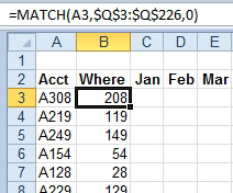
Strategy: Add a soon-to-be-hidden column called Where and put a MATCH formula there to figure out where the product is located. Once you know where the product, use 12 columns of INDEX to return the columns from the lookup table.

This figure shows the Where column. This column takes about as long to calculate as the January VLOOKUP would take.

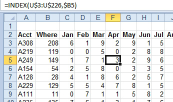
Now that you have the MATCH running the Where column, you can build an incredibly simple INDEX function. It is interesting to consider the placement of dollar signs in this formula.

Add a Where column. Do =MATCH(A3,Q3:Q226,0) to find the row number associated with the account in A3. — Figure 427. Product A308 is found in the 208th row of the lookup table.

1. In cell C3, enter =INDEX(R$3:R$226,$B3). You are using $ before 3 and 226 to make sure that the lookup table is always pointing from row 3 to row 226. However, you are not using dollar signs before column R. R3:R226 contains the January values. When you copy this formula to the right one cell, the lookup table shifts to the February column and points to S$3:S$226. The second argument of INDEX uses a single dollar sign before column B. This way, as you copy the formula, it is always pointing back to column B to get the row number of this product in the lookup table.
2. Copy C3 to D3:N3.
3. Select C3:N3.
4. Copy it down to all rows by double-clicking the fill handle in the lower right corner of N3.
5. Hide column B.

Solving the 12 columns of VLOOKUP problem with one column of MATCH (labeled Where) and then 12 columns of INDEX that point to the results of the MATCH. — Figure 428. This table is 10 times faster than all VLOOKUPs.

The MATCH with INDEX solution shown here solves the whole problem of editing the third argument of the VLOOKUP for each column. Two simple formulas create the entire table. Plus, it runs much faster that using 12 columns of VLOOKUP.

I’ve met people who tell me that they have quit using VLOOKUP and rely entirely on MATCH and INDEX.

This article is an excerpt from Power Excel With MrExcel

Title photo by Jason Leung on Unsplash