Excel 2024: Use the LET Function to Re-Use Variables in a Formula

The LET function debuted during 2020 for Microsoft 365 Subscribers. There are all sorts of calculations in Excel that can benefit from re-using an intermediate calculation.

Someone e-mailed me and needed a formula to find the next-to-last word in a series of phrases stored in column A. Each cell might have anywhere from 5 to 10 words. I know that I can solve this type of problem, but I know the solution will have a lot of parts. So, my strategy is to insert a bunch of columns and work it out, piece by piece.

The solution requires me to count the words by taking the LEN of the phrase and then the LEN of the phrase with the spaces removed. Once you know the number of words, you can change the correct space to a ^ and then use FIND to isolate the location of the caret. Once you use MID to get the text after the caret, you find the space between the last and next-to-last word and use LEFT. While each step is simple, knowing how to put all of those together is tricky.

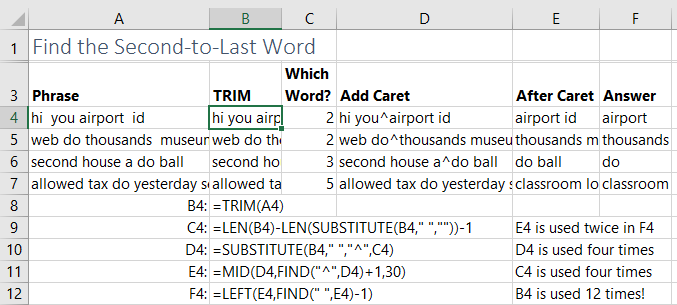
In the figure below, I have built the solution using five formulas. It is working and I could likely explain it to anyone who uses Excel 10 hours a week.

However, I've also learned that some people just want the formula to solve this, and they don't want to know how it works. Those people want the whole formula to be in a single cell.

At this point, I often try to merge everything into a single formula. The formula in cell F4 refers to the formula in E4 twice. Select E4. Using the mouse in the Formula Bar, carefully select everything after the equals sign and then copy it. Edit the original formula in F4. Select the characters E4 in the formula and use CTRL+V to paste to replace E4 with the actual formula from E4. Continue in this fashion until you have a single formula.

The formula keeps growing, and eventually the B4 formula of TRIM(A4) appears a total of 12 times in the final formula. Excel has to perform the TRIM operation 12 times for each cell. Explaining this formula to someone else will be difficult, if not impossible.

=LEFT(MID(SUBSTITUTE(TRIM(A4)," ","^",LEN(TRIM(A4))-LEN(SUBSTITUTE(TRIM(A4)," ",""))-1), FIND("^",SUBSTITUTE(TRIM(A4)," ","^",LEN(TRIM(A4))-LEN(SUBSTITUTE(TRIM(A4)," ",""))-1))+1,30),FIND(" ",MID(SUBSTITUTE(TRIM(A4)," ","^",LEN(TRIM(A4))-LEN(SUBSTITUTE(TRIM(A4), " ",""))-1),FIND("^",SUBSTITUTE(TRIM(A4)," ","^",LEN(TRIM(A4))-LEN(SUBSTITUTE(TRIM(A4), " ",""))-1))+1,30))-1)

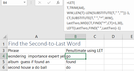
This is where the LET function helps. The LET function starts out with pairs of arguments where you give a variable name and the definition for that variable. The calculation for the second variable can re-use the logic assigned to the first variable. The final argument in the function is the calculation returned to the cell.

You can plan out your LET function as shown here:

And then wrap that logic in the LET function:

---

---

The best practice for LET is to use Alt+Enter to go to a new line in the formula bar after each pair of arguments. This makes the formula easier to read.

The LET function will simplify an entire class of problems where you need to repeatedly refer to an earlier component later in the formula.