Excel 2024: Sorting with a Formula
July 31, 2024 - by Bill Jelen

Sorting data in Excel is easy. Unless, you are building a dashboard for your manager's manager. You can't ask that person to select C3, go to the Data tab and click the AZ button every time they want an updated report. The new SORT and SORTBY functions allow you to easily sort with a formula.
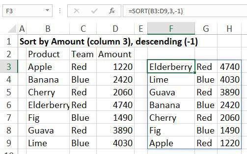
You can pass three arguments to the SORT function. The first is the range to be sorted. Leave the headings out of this argument. Next, which column do you want to sort by. If your data is in B:D and you want to sort by column D, you would specify column 3 as the sort column. The third argument is a 1 for ascending or -1 for descending.
In this figure, the data is sorted by Amount descending:

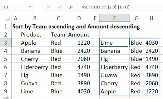
What if you want to do a two-level sort? You can specify an array constant for both the second and third argument. In this case, the data is sorted by Team ascending and Amount descending. For the sort column, specify {2;3}. For the sort order, specify {1;-1}.

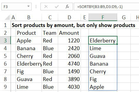
The Excel Calc team also gave you the SORTBY function. Say you want to return a list of products but not the associated amounts. You want the products to be sorted by the amount. The formula below says to return the products from B3:B9 sorted descending by the amounts in D3:D9.

Bonus Tip: Sort into a Random Sequence
Why would you need to sort randomly? Perhaps you are picking the lucky winner of a free Thanksgiving turkey. Or the unlucky winner of the quarterly drug screening. Use SORTBY and specify the list of employees as the first argument. For the second argument, use RANDARRAY(N) where N is the number of employees. Every time you press F9, the results in column D will sort again.

This article is an excerpt from MrExcel 2024 Igniting Excel
Title photo by Kier in Sight Archives on Unsplash
