Excel 2024: See All Formulas at Once

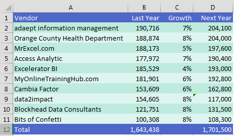
You inherit a spreadsheet from a former co-worker and you need to figure out how the calculations work. You could visit each cell, one at a time, and look at the formula in the formula bar. Or you could quickly toggle between pressing F2 and Esc to see the formula right in the cell.

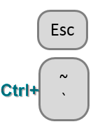
But there is a faster way. On most U.S. keyboards, just below the Esc key is a key with two accent characters: the tilde from Spanish and the grave accent from French. It is an odd key. I don't know how I would ever use this key to actually type piñata or frère .

If you hold down Ctrl and the grave accent, you toggle into something called Show Formulas mode. Each column gets wider, and you see all of the formulas.

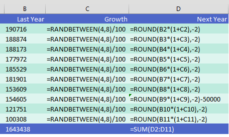
This gives you a view of all the formulas at once. It is great for spotting plug numbers (D9) or when someone added the totals with a calculator and typed the number instead of using =SUM(). You can see that the co-worker left RANDBETWEEN functions in this model.

Bonus Tip: Highlight All Formula Cells

If you are going to be auditing the worksheet, it would help to mark all of the formula cells. Here are the steps:

1. Select any blank cell in the worksheet.

2. Choose Home, Find & Select, Formulas.

3. All of the formula cells will be selected. Mark them in a different font color, or, heck, use Home, Cell Styles, Calculation.

To mark all of the input cells, use Home, Find & Select, Go To Special, Constants. I prefer to then uncheck Text, Logical, and Errors, leaving only the numeric constants. Click OK in the Go To Special dialog.

Why Is the F1 Key Missing from Your Keyboard?

Twice I have served as a judge for the ModelOff Financial Modeling Championships in New York. On my first visit, I was watching contestant Martijn Reekers work in Excel. He was constantly pressing F2 and Esc with his left hand. His right hand was on the arrow keys, swiftly moving from cell to cell. F2 puts a cell in Edit mode so you can see the formula in the cell. Esc exits Edit mode and shows you the number. Martijn would press F2 and Esc at least three times every second.

But here is the funny part: What dangerous key is between F2 and Esc? F1. If you accidentally press F1, you will have a 10-second delay while Excel loads online Help. If you are analyzing three cells a second, a 10-second delay is a disaster. You might as well go to lunch. So, Martijn had pried the F1 key from his keyboard so he would never accidentally press it.

Photo Credit: Mary Ellen Jelen

Bonus Tip: Trace Precedents to See What Cells Flow into a Formula

If you need to see which cells flow into a formula, you can use the Trace Precedents command in the Formula Auditing group on the Formulas tab. In the following figure, select D6. Choose Trace Precedents. Blue lines will draw to each cell referenced by the formula in D6. The dotted line leading to a symbol in B4 means there is at least one precedent on another worksheet. If you double-click the dotted line, Excel shows you a list of the off-sheet precedents. If you stay in cell D6 and choose Trace Precedents a few more times, you will see the second-level precedents, then the third-level precedents, and so on. When you are done, click Remove Arrows.

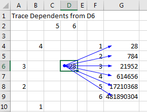
Bonus Tip: See Which Cells Depend on the Current Cell

Sometimes you have the opposite problem: You want to see which cells rely on the value in the current cell. Choose any cell and click Trace Dependents to see which cells directly refer to the active cell.