Excel 2024: Replace a Pivot Table with 3 Dynamic Arrays

August 15, 2024 - by Bill Jelen

As the co-author of Pivot Table Data Crunching, I love a good pivot table. But Excel Project Manager Joe McDaid and Excel MVP Roger Govier both pointed out that the three formulas shown here simulate a pivot table and do not have to be refreshed.

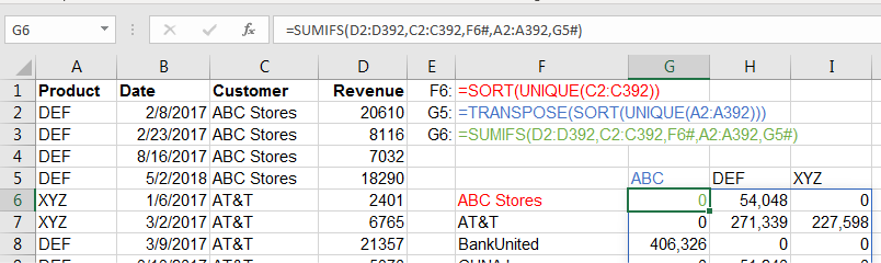
To build the report, =SORT(UNIQUE(C2:C392)) provides a vertical list of customers starting in F6. Then, =TRANSPOSE(SORT(UNIQUE(A2:A392))) provides a horizontal list of products starting in G5.

When you specify F6# and G5# in arguments of SUMIFS, Excel returns a two-dimensional result: =SUMIFS(D2:D392,C2:C392,F6#,A2:A392,G5#).

Four columns of source data: Product, Date, Customer and Revenue. Headings are in row 1, data is rows 2:392. =SORT(UNIQUE(C2:C392)) gets a vertical sorted list of customers starting in F7. Then, =TRANSPOSE(SORT(UNIQUE(A2:A392))) gets a horizontal list of products in G5. Finally, =SUMIFS(D2:D392,C2:C392,F6#,A2:A392,G5#) in G6 fills in the Revenue amount for each combination of Customer and Product.

This article is an excerpt from MrExcel 2024 Igniting Excel

Title photo by Lukas Blazek on Unsplash