Excel 2024: Pivot Table with Sum and Average Total Rows (MDX)

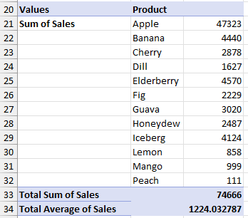
Check out this impossible pivot table. Details for Sum of Sales. Total for Sum of Sales. Then, without any details for Average of Sales, a Total row for Average of Sales. Notice that there are no hidden rows between row 33 and 34.

In the past, in my live seminars, I've done this using a Data Model pivot table and an obscure setting to Create a Set Based on Row Items. This method is fragile and will break if a new product is introduced. The method in this edition of the book involves editing the MDX (which stands for Multidimensional Expressions). The steps are pretty easy.

1. Your data set must be a table. Select one cell in the data and press Ctrl+T. Make sure to choose My Data Has Headers and click OK.

2. Excel gives the table a name like Table1 or something like that. On the left side of Table Tools, type a new name of Data

3. From inside the Data table, choose Insert, Pivot Table.

4. In the Pivottable dialog box, choose Add This Data To The Data Model. This setting enables MDX to work.

5. Drag Product to the Rows area of the pivot table. Drag Sales to the Values area. Drag Sales a second time to the Values area.

6. There are two headings: Sum of Sales and Sum of Sales 2. Double-click the heading for Sum of Sales 2 to open the Value Field Settings. Change the calculation from Sum to Average.

7. This is very important: Change the Custom Name from Average of Sales 2 to Average of Sales.

8. Click OK to close the Value Settings dialog

9. Look in the PivotTable Fields pane. There is a new tile in the Columns area called Sigma Values. It does not have the word Sigma... it has the Sigma symbol - a funny-looking angular capital E. Drag this tile and drop it above the Product tile in the Rows area. If you did this correctly, your pivot table now has 12 rows of Sum of Sales followed by 12 rows of Average of Sales, followed by two grand total rows. If it is not matching, it is time to watch Episode 2547.

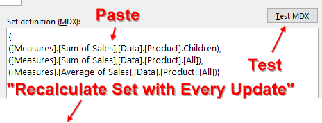
10. Open the workbook for this chapter. Copy the red text from the text box. Or, get ready to type all of this:

11. On the PivotTable Analyze tab, open the drop-down for Fields Items and Sets. Choose Manage Sets.

12. In the Set Manager dialog, open the drop-down for New and choose Create Set from MDX.

13. Paste the four lines of MDX code from above. Click Test MDX to make sure it is valid.

14. At the bottom of the dialog, choose Recalculate Set With Every Update.

15. Click OK to close this dialog.

16. Click Close to close the Set Manager dialog. You will now see a new checkbox at the top of the PivotTable Fields pane for Set 1.

17. Uncheck Product and Sales from the PivotTable Fields pane. Choose Set 1. Your pivot table will now look like the pivot table at the beginning of this topic.