
Excel 2024: Geography, Exchange Rate & Stock Data Types in Excel
July 22, 2024 - by Bill Jelen

In the past, Excel did not really handle data types. Yes, you could format some cells as Date or Text, but the new data types provide a whole new entry point for new data types now and in the future.
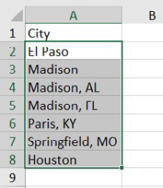
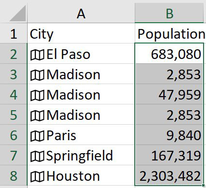
Start with a column of City names. For large cities like Madison Wisconsin, you can just put Madison. For smaller towns, you might enter Madison, FL.
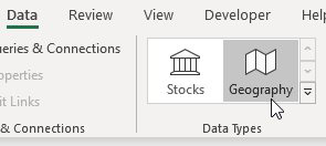
From the Data tab, select Geography.
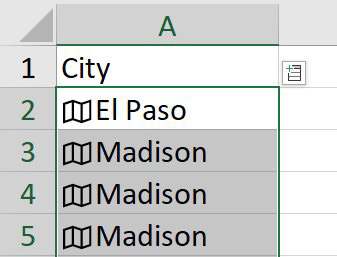
Excel searches the Internet and finds a city for each cell. A folded map appears next to each cell. Notice that you lose the state that was in the original cell.
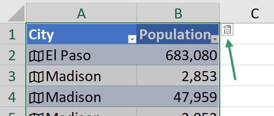
Click on the Map icon and a data card appears with information about the city.
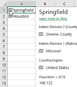
The best part: for any data in the card, you can use a formula to pull that data into a cell. Enter =A2.Population in cell B2 and Excel returns the population of El Paso. Double click the Fill Handle in B2 and Excel returns the population for each city.
Caution: These new formulas might return a #FIELD! error. This means, Excel (or more correctly Bing), does not know the answer to this yet, but it may do so at some time in the future. It is not an error with the formula or the table, just a lack of knowledge currently.
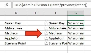
Here is a great tip: Excel uses the context of other cells around the value to try to figure out ambiguous entries. In the following image, because Madison is in the middle of other Wisconsin cities, Excel will automatically choose Madison Wisconsin.
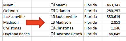
If you type Madison in a column that has Florida cities, Excel will correctly figure out that you want Madison Florida, even though it is smaller than the capital city of Wisconsin.
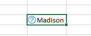
If you simply type Madison in a cell without any other values above or below it, Excel won't choose any of the towns named Madison. Instead of a map icon, you will have a circled question mark. The Data Selector pane will appear to allow you to choose which Madison you want.
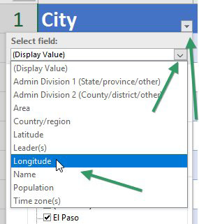
The Geography and Stock data types have extra features if you format as a table using Ctrl+T.
A new Add Data icon appears to the right of the heading. Use this drop-down menu to add fields without having to type the formulas. Clicking the icon will enter the formula for you.
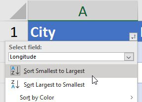
You can also sort the data by any field, even if it is not in the Excel grid. Open the drop-down menu for the City column. Use the new Display Field drop-down to choose Longitude.
With Longitude selected, choose sort Smallest to Largest.
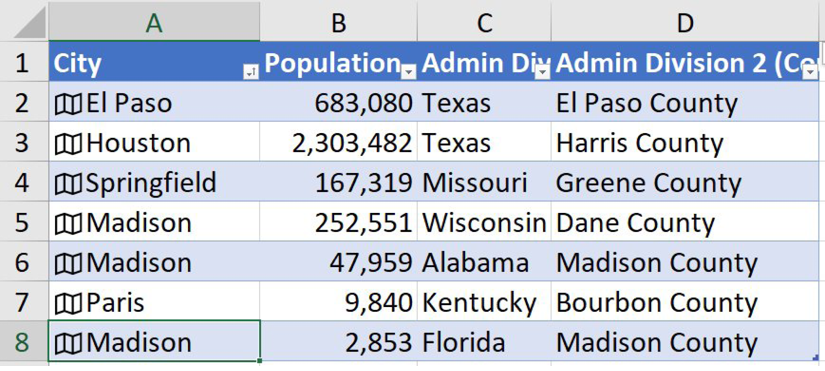
The result: data is sorted west to east.
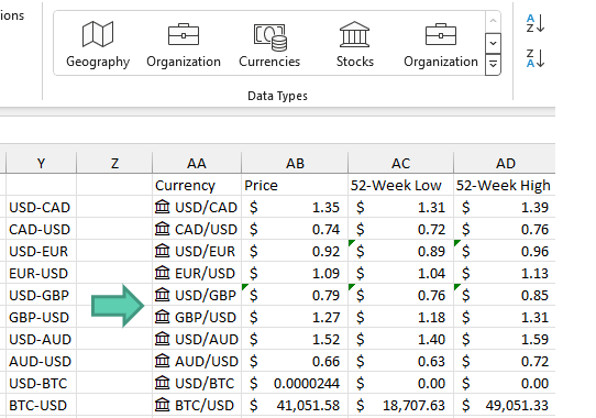
Support for exchange rates appeared in early 2019. While it initially was accessed by using the Stocks icon, it now has it's own Currency icon in the gallery. Enter currency pairs such as USD-CAD for U.S. Dollar to Canadian Dollar. Use the Price field for the current exchange rate.
Bonus Tip: Use Data, Refresh All to Update Stock Data
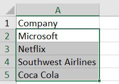
Another data type available is Stock data. Enter some publicly held companies:
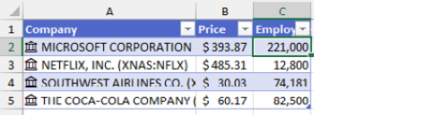
Choose, Data, Stocks. An icon of a building with Roman columns should appear next to each company You can add fields such as Number of Employees, Price, Volume, High, Low, Previous Close.
In contrast to Geography, where population might only be updated once a year, the stock price will be constantly changing throughout the trading day. Rather than go out to the Internet with every recalc, Excel will only updated the data from these Linked Data Types when you choose Refresh.
One easy way to update the stock prices is to use the Refresh All icon on the Data tab.
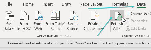
As the name implies, Refresh All will update everything in your workbook, including any Power Query data connections which might take a long time to update. If you want to only refresh the current block of linked data, right-click on A2, choose Data Types, Refresh.
At some point in 2021, a new setting will allow Stock Data Types to update every five minutes.
Right-click any cell with a Stock Data Type. Choose Data Type, Refresh Settings.
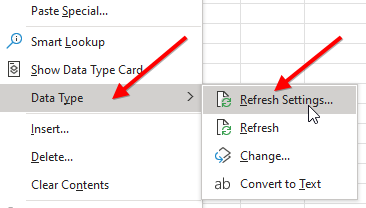
|
In the Data Types Refresh Settings, click the Stocks chevron to open the options. Select Automatically Update Every 5 Minutes. Note Yes, the choices here are limited. What if you want to refresh every one minute or every 10 minutes? Too bad. Getting the choice to refresh every five minutes is better than the two years when you had to manually refresh. |
 |
The Stock data type only delivers the current day's stock price. For stock history, see the STOCKHISTORY function.
This article is an excerpt from MrExcel 2024 Igniting Excel
Title photo by AbsolutVision on Unsplash