Excel 2024: Find Largest Value That Meets One or More Criteria

October 11, 2024 - by Bill Jelen

One of the new Microsoft 365 functions added in February 2016 is the MAXIFS function. This function, which is similar to SUMIFS, finds the largest value that meets one or more criteria: You can either hard-code the criterion as in row 7 below or point to cells as in row 9. A similar MINIFS function finds the smallest value that meets one or more criteria.

Amounts appears in D12:D125. To get the Largest, use =MAX($D$12:$D$125). To get the 2nd Largest, use =LARGE($D$12:$D$125,2). To get the 3rd Largest, use =LARGE($D$12:$D$125,3). To get the 3rd Smallest, use =SMALL($D$12:$D$125,3). To get the 2nd Smallest, use =SMALL($D$12:$D$125,2). To get the Smallest, use =MIN($D$12:$D$125). To get the Smallest Widget, use =MINIFS($D$12:$D$125,$B$12:$B$125,"Widget"), To get the Largest with 2 Criteria entered in B8:C8, use =MAXIFS($D$12:$D$125,$B$12:$B$125,B8,$C$12:$C$125,C8)

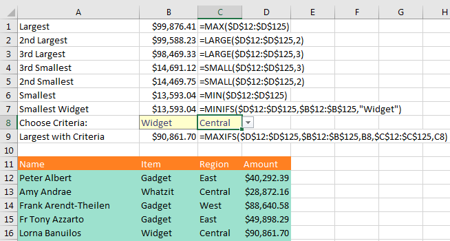
While most people have probably heard of MAX and MIN, but how do you find the second largest value? Use LARGE (rows 2 and 3) or SMALL (rows 4 and 5).

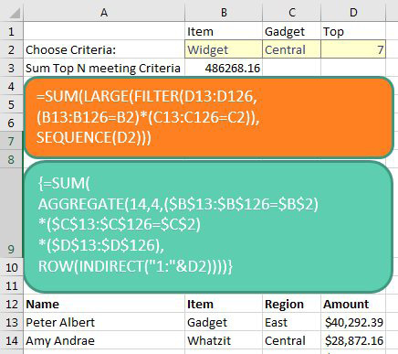
What if you need to sum the top seven values that meet criteria? The orange box below shows how to solve with the new Dynamic Arrays. The green box is the Ctrl+Shift+Enter formula required previously.

Before Dynamic Arrays, you would use: '{=SUM(
AGGREGATE(14,4,($B$13:$B$126=$B$2)
*($C$13:$C$126=$C$2)
*($D$13:$D$126),
ROW(INDIRECT("1:"&D2))))}.
With Dynamic Arrays, the formula is =SUM(LARGE(FILTER(D13:D126,(B13:B126=B2)*(C13:C126=C21)),SEQUENCE(D2)))

Bonus Tip: Concatenate a Range by Using TEXTJOIN

My favorite new calculation function in Microsoft 365 is TEXTJOIN. What if you needed to concatenate all of the names in A1:A10? The formula =A1&A2&A3&A4&A5&A6&A7&A8&A9&A10 would jam everyone together like AndyBobCaroleDaleEdFloGloriaHelenIkeJill. By using TEXTJOIN, you can specify a delimiter such as ", ". The second argument lets you specify if blank cells should be ignored. =TEXTJOIN(", ",True,A1:A10) would produce Andy, Bob, Carole, and so on.

To get a list of all people in A10:A18 with commas in between, use =TEXTJOIN(", ",TRUE,$A$10:$A$18). To limit to only the people where RSVP=Yes in column B, use: =TEXTJOIN(", ",TRUE,IF(B10:B18="Yes",A10:A18,"")) with Ctrl+Shift+Enter.

Tip

TEXTJOIN works with arrays. The array formula shown in A7 uses a criterion to find only the people who answered Yes. Make sure to hold down Ctrl + Shift while pressing Enter to accept this formula. The alternate formula shown in A8 uses the Dynamic Array FILTER function and does not require Ctrl+Shift+Enter.

This article is an excerpt from MrExcel 2024 Igniting Excel

Title photo by frank mckenna on Unsplash