Excel 2024: Discover New Functions by Using fx
June 20, 2024 - by Bill Jelen

There are 509 functions in Excel. I have room for only 155 tips this book, so there is no way I can cover them all. But instead of taking 450 pages to describe every function, I am going to teach you how to find the function that you need.
The Excel 2007 formulas tab introduced a huge fx Insert Function icon. But you don't need to use the one on the Formulas tab; the same icon has been to the left of the formula bar ever since I can remember.
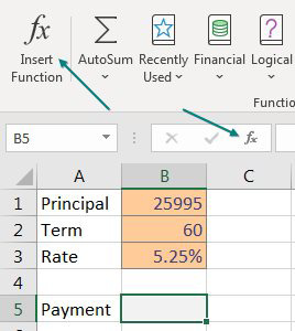
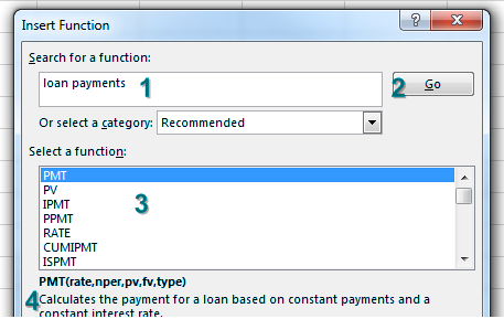
If you are trying to figure out how to calculate a loan payment, the Insert Function dialog will help. Click the icon next to the formula bar. In the Search for a Function box, type what you are trying to do. Click Go. The Select a Function box shows functions related to your search term. Click on a function in that box to see the description at the bottom of the dialog.
Caution: A change in Excel Help caused the search to return less results starting in 2019.
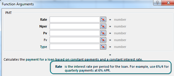
When you find the correct function and click OK, Excel takes you into the Function Arguments dialog. This is an amazing tool when you are new to a function. As you click in each argument box, help appears at the bottom of the window, with specifics on that argument.
Personally, I could never get the PMT function to work correctly because I always forgot that the rate had to be the interest rate per period. Instead of pointing to the 5.25% in B3, you have to point to B3/12. Below, the help for Nper explains that it is the total number of payments for the loan, also known as the term, from B2.
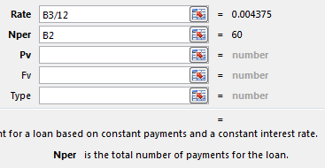
PV is the loan amount. Since I never write a check for negative $493, I want the answer from PMT to be positive instead of negative. That is why I always use -B1 for the PV argument. If you use B1 instead, you will get the correct $493.54065 answer, but it will appear as negative in your worksheet. Think of the original $25,995 as money leaving the bank; that is why the PV is negative.
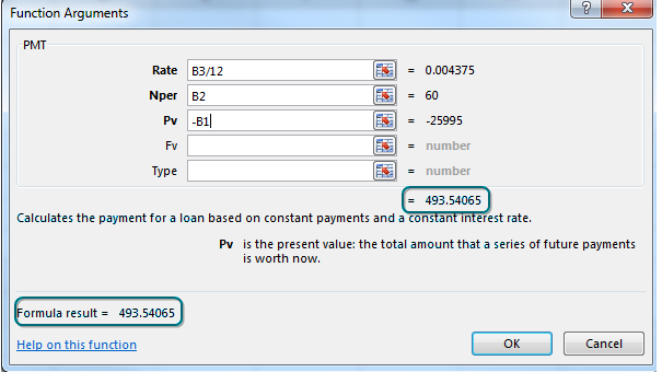
Notice in the above figure that three argument names are bold. These are the required arguments.
Once you finish the required arguments, the Function Arguments dialog shows you the answer in two places. I always use this as a sanity check. Does this answer sound like a typical car payment?
This one topic really covered three things: how to calculate a loan payment, how to use the fx icon to discover new functions, and how to use the Function Arguments dialog to get help on any function.
If you are in a situation where you remember the function name but still want to use the Function Arguments dialog, type =PMT( with the opening parenthesis and then press Ctrl+A. If you press Ctrl+Shift+A, Excel will insert the names of the arguments into the formula.

Thanks to Excel MVP Nabil Mourad from OfficeInstructor.com for the Ctrl+Shift+A technique.
This article is an excerpt from MrExcel 2024 Igniting Excel
Title photo by fernando bacheschi on Unsplash
