Excel 2024: Calculate Percent of Total with PERCENTOF Function

August 22, 2024 - by Bill Jelen

When the Excel team created PIVOTBY, they wanted to be able to show percent of total within the pivot table. One of the side benefits is that you get a new PIVOTBY function.

The syntax is simple: =PERCENTOF(data_subset,data_all)

In this image, the formula in D6 is asking for the 3809 divided by the total of sales in C4:C9.

Bonus Tip: Replace Ctrl+Shift+Enter with Dynamic Arrays.

Before dynamic arrays, people would use these crazy Ctrl+Shift+Enter formulas.

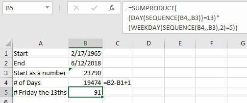
Say that you have a friend who is superstitious about Friday the 13th. You want to illustrate how many Friday the 13ths your friend has lived through. Before Dynamic Arrays, you would have to use the formula below.

The same formula after dynamic arrays is still complicated, but less intimidating:

With dynamic arrays, the formula is =SUMPRODUCT(
(DAY(SEQUENCE(B4,,B3))=13)*
(WEEKDAY(SEQUENCE(B4,,B3),2)=5))
entered without Ctrl+Shift+Enter. — With dynamic arrays, the formula is =SUMPRODUCT( (DAY(SEQUENCE(B4,,B3))=13)* (WEEKDAY(SEQUENCE(B4,,B3),2)=5)) entered without Ctrl+Shift+Enter.

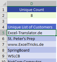
Another example from Mike Girvin's Ctrl+Shift+Enter book is to get a unique list.

A helper formula in D2 counts the number of unique items in a list. Then, a formula returns the unique list in D5. See the next screenshot for the formula.

Here is the formula. I won't try to explain it to you.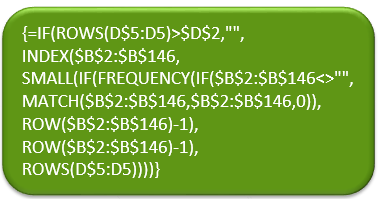

This was the insane formula to get the unique list before Dynamic Arrays: =IF(ROWS(D$5:D5)>$D$2,"",
INDEX($B$2:$B$146,
SMALL(IF(FREQUENCY(IF($B$2:$B$146<>"",
MATCH($B$2:$B$146,$B$2:$B$146,0)),
ROW($B$2:$B$146)-1),
ROW($B$2:$B$146)-1),
ROWS(D$5:D5)))) — This was the insane formula to get the unique list before Dynamic Arrays: =IF(ROWS(D$5:D5)>$D$2,"", INDEX($B$2:$B$146, SMALL(IF(FREQUENCY(IF($B$2:$B$146<>"", MATCH($B$2:$B$146,$B$2:$B$146,0)), ROW($B$2:$B$146)-1), ROW($B$2:$B$146)-1), ROWS(D$5:D5))))

The replacement formula with dynamic arrays is =UNIQUE(B2:B146).

This article is an excerpt from MrExcel 2024 Igniting Excel

Title photo by Karim MANJRA on Unsplash