Excel 2024: Use Function Arguments for Nested Functions


June 24, 2024 - by

Excel 2024: Use Function Arguments for Nested Functions

The Function Arguments dialog shown above is cool, but in real life, when you have to nest functions, how would you use this dialog?

Say that you want to build a formula to do a two-way lookup:

=INDEX(B2:E16,MATCH(G2,A2:A16,0),MATCH(H2,B1:E1,0))

The lookup table has accounts down the left side and month across the top. Someone will enter an Account in G2 and a Month in H2. The result needs to appear in I2 using the formula described just before this image.

You would start out using the Function Arguments dialog box for INDEX. In the Row_num argument box, type MATCH(. Using the mouse, go up to the formula bar and click anywhere inside the word MATCH.


Start out using the Function Arguments dialog box for INDEX. Enter B2:F16 as the array. Tab into the Row Num box. Type MATCH( in the box. Then, look up in the formula bar. Using the mouse, click inside the MATCH function. The Function Arguments will change to the MATCH function with the correct arguments for MATCH.

Start out using the Function Arguments dialog box for INDEX. Enter B2:F16 as the array. Tab into the Row Num box. Type MATCH( in the box. Then, look up in the formula bar. Using the mouse, click inside the MATCH function. The Function Arguments will change to the MATCH function with the correct arguments for MATCH.

Caution: Don't click the formula in the cell. You have to click the formula in the formula bar.

The Function Arguments dialog switches over to MATCH. When you are finished building the MATCH function, go up to the formula bar and click anywhere in the word INDEX.
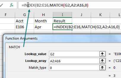
After entering the three arguments for MATCH, you need to return to the INDEX version of Function Arguments. Reach up to the Formula Bar and click inside the word INDEX.

Repeat these steps to build the MATCH in the third argument of INDEX. Make sure to click back in the word INDEX in the formula bar when you are done with the second MATCH.
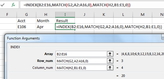
At this point, you have successfully entered a formula using one INDEX and two MATCH functions, all using the Function Arguments dialog.


It turns out that the Function Arguments dialog can be fooled into building an invalid function. Type a well-formed but nonsensical function in the formula bar. Using the mouse, click inside the fake function name in the formula bar and click the fx icon.
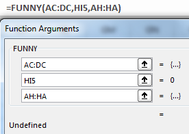
If you type a nonsensical function such as =FUNNY(AC:DC,HI5,AH:HA) and open the Function Arguments, it will allow you to edit the three arguments, although it does not know the name or the help topic for any of them.

Thanks to Tony DeJonker, Cat Parkinson, & Geoff in Huntsville for suggesting the Function Arguments dialog trick.


This article is an excerpt from MrExcel 2024 Igniting Excel

Title photo by Abhijit Sinha on Unsplash