Embed a Small Lookup Table In Formula
May 05, 2022 - by Bill Jelen

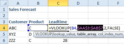
Problem: I have a small 5-row lookup table hidden out in column AA:AB. The sales reps who use the spreadsheet might inadvertently delete a row in their data, deleting the lookup table. Can I put the lookup table somewhere that they won’t destroy it?
Strategy: One solution is to move the lookup table to a new worksheet and hide the worksheet. However, if the lookup table is small, you can embed it right in the VLOOKUP formula. Follow these steps:
1. Select the cell with the
VLOOKUPformula.2. Press F2 to put the cell in edit mode
-
3. Select the characters that represent the lookup table.

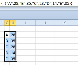
4. Press F9. This calculates the selected portion of the formula. In this case, it puts
{“A”,28;”B”,35;”C”,28;”D”,14;”E”,35}into the formula.

5. Enter the formula. Copy it down to the other rows. You can now safely delete the lookup table.
It helps to understand Excel’s array syntax. The curly braces indicate that this is an array. Each comma means you should move to a new column. Each semicolon means that you should move to a new row.
Gotcha: It is difficult to later edit the table. You can try to puzzle it out by staring at the commas and semi-colons in the formula bar. Or, you can copy the array and put it back in the worksheet. You have to follow these steps:
1. Select the array from the formula, including the curly braces.
2. Ctrl+C to copy the characters from the clipboard.
3. Select a five-row by 2 column blank section of the spreadsheet.
4. Type an equals sign. Press Ctrl+V. Press Ctrl+Shift+Enter. Excel will put the array back into the worksheet as an array formula. This looks OK, but you can not edit individual cells in the range.

5. With the entire range selected, do a Copy and then Paste Values. You can now edit individual cells in the table.
This article is an excerpt from Power Excel With MrExcel
Title photo by Gabriella Clare Marino on Unsplash
