Deal with Data in Which Each Record Takes Five Physical Rows

November 03, 2022 - by Bill Jelen

Problem: Sometime, back in the days of COBOL, a programmer was dealing with the constraints of the physical width of a page. The programmer built a report in which each record actually took up five lines of the report. I want to be able to analyze this data in Excel.

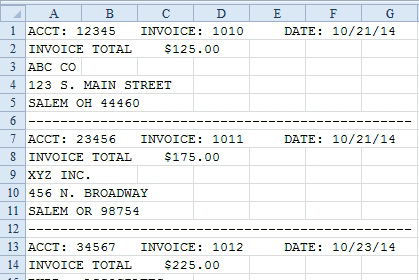
An ugly data format where each "record" takes up six physical rows in the worksheet. You can always count on City, State, Zip in the fifth row of each record. — Figure 793. Transform this frustrating data set.

Strategy: Your goal is to get the data back into one row per record. This process involves adding two new columns, Group and Sequence:

1. Add a new row 1. Insert two new columns, A and B. Add the headings Group, Seq, and Text in A1:C1.

Add two new columns to the left of the data, one for Group and one for Sequence. — Figure 794. Add two new columns.

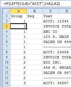
2. In column A, assign a group number to each logical record. One way to do this is to check to see if the first four characters of column C are ACCT. If they are, add 1 to the group number. In A2, enter the number 1. In A3, enter the formula =IF(LEFT(C3,4)=”ACCT”,1+A2,A2). (This is similar to the formula from “Add a Group Number to Each Set of Records That Has a Unique Customer Number”.) Copy it down to all the rows. Excel will assign a group number to each logical group of records.

The formula in A3 is =IF(LEFT(C3,4)="ACCT",1+A2,A2). This says if we are at the top of the next record, add one to the previous group number. Otherwise, copy the Group Number from above. The figure shows this working with the first six rows labeled 1, then six rows labeled 2, and so on. — Figure 795. Use the IF function.

3. Design a formula for a sequence number. To do this, in cell B2, enter the formula =IF(A2=A1,B1+1,1). (This formula is like the one from “Number Each Record for a Customer, Starting at 1 for a New Customer”) Copy this down. This formula will number each record in the group. It should ensure that all the account numbers are on a Sequence 1 record.

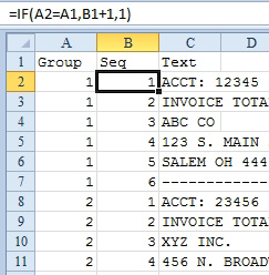
The formula for Sequence in B2 is =IF(A2=A1,B1+1,1). This says: If this Group equals the previous group, then add one to the previous sequence. Otherwise, reset the sequence to 1. — Figure 796. Formula for sequence number.

4. (This step is critical.) Copy the formulas in columns A and B and paste them back, using Home, Paste dropdown, Paste Values to ensure that you can safely sort the data.
5. Sort the data by the sequence number in column B. Your data will look like this.

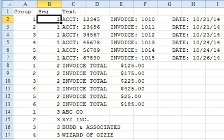
With the Group and Sequence changed to values, you can sort by Sequence to get all of the rows that Have Account, Invoice, and Date in one section, followed by group 2 with Invoice Total, followed by Group 3 with Customer Name. — Figure 797. Sort the data into record types.

You have now managed to intelligently segregate the data so that all similar records are together. The contiguous range C2:C7 contains all the first rows from each record. Each of the line 1 records has three fields that really should be parsed into three separate columns. You can easily do this parsing with the Text to Columns Wizard.

6. Select cells C2:C7. Select Data, Text to Columns to open the Convert Text to Columns Wizard. Select Fixed Width. Click Next.
7. Excel should properly guess where your columns are. Click Next.
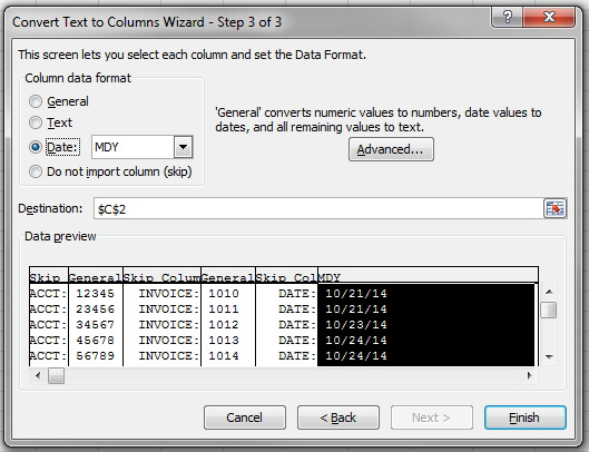
8. Choose the heading for each column and define a data format. You don’t really need the word ACCT each time, so choose to skip the first, third, and fifth fields. Make the sixth field a date. When your information looks as shown below, click Finish. You will have data in three columns of Group 1.

Select only the data for Records 1. Use Text to Columns, Fixed Width. In Step 3, liberal use of Skip Column will get rid of the text headings that you do not need. — Figure 798. In Step 3, skip columns 1, 3, and 5. Choose Date for col. 6.

9. Change the heading in C1 to Acct, the heading in D1 to Inv, and the heading in E1 to Date.
10. Select and cut A8:C13 and paste into F2.
11. Delete Group & Seq from F & G.
12. Add the heading of Inv $ to F1.
13. Select F2:F6 and choose Data, Text to Columns. In Step 1 of the wizard, select Fixed Width and click Next. In Step 2 of the wizard, Excel offers to split your data into three fields. There is no need to have one column for the word Invoice and another column for the word Total.

For Section 2, the Text to Column tries to create three columns that will say:
Invoice
Total
and then the Actual Numeric total. — Figure 799. Excel suggests an extra column.

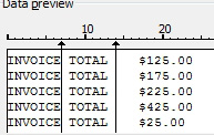
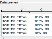
14. Double-click the line between Invoice and Total to delete it.

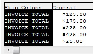
Double click the line between Invoice and Total to combine Invoice Total into a single column. — Figure 800. Double-click the extra line to delete it.

15. In Step 3 of the wizard, choose to skip the field that contains Invoice Total. Click Finish.

In Step 3 of the Text to Columns Wizard, choose Skip Column for the column that would have said Invoice Total. This will leave only the numeric total left. — Figure 801. Skip the field label.

16. Records for Groups 3 through 5 only have a single field without a heading. Copy C14:C19 to G2. Add a heading of Company.
17. Copy Group 4’s column C cells to H2. Add a heading of Address.
18. Copy Group 5’s column C cells to I2. Add a heading of City ST Zip.
19. Because the Group 6 records have no data—they are just dashed lines—delete these rows.

You now have all the fields, one line per record.

20. Delete the columns extra columns A& B.

Results: You now have a sortable, filterable, and reportable version of the original data set. Each record consists of one row in Excel.

You can Cut all of the invoice totals and paste to the right of the section 1 results. For each additional section, cut and paste the results to the right. This now shows an eight column data set with Acct, Invoice, Date, Invoice Total, Company, Street, City, State, and Zip. — Figure 802. You can now sort and analyze this data.

This article is an excerpt from Power Excel With MrExcel

Title photo by Kelly Sikkema on Unsplash