Ctrl+T Makes VLOOKUP Better
August 11, 2017 - by Bill Jelen

In the last episode, Ctrl + T made the pivot table source expand
In almost every seminar, someone asks why their pivot tables default to counting a numeric field instead of summing. There are two possible answers: Either there are a few blank cells in the numeric column, or the person is selecting entire columns in the data set (such as A:C instead of A1:C16).
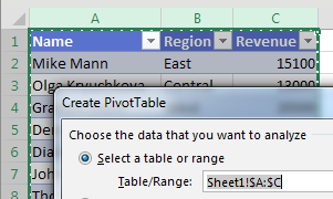
I understand the logic behind the second possibility. If you choose all of columns A:C and you later want to add more records below the data, it takes only a simple Refresh to add the new data instead of having to find the Change Data Source icon. In the past, this made sense. But today, Change Data Source is right next to the Refresh button and not hard to find. Plus, there is a workaround in the Ctrl + T Table.
When you choose your data set and select Format as Table by using Ctrl + T, the pivot table source will grow as the table grows. You can even do this retroactively, after the pivot table exists.
This figure shows a data set and a pivot table. The pivot table source is A1:C16.
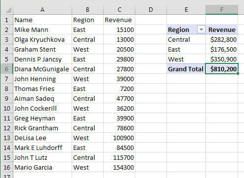
You want to be able to easily add new data below the pivot table.
Select one cell in the data and press Ctrl + T. Make sure that My Table Has Headers is checked in the Create Table dialog and click OK.
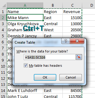
Some nice formatting is applied to the data set. But the formatting is not the important part.
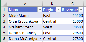
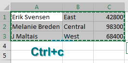
You have some new records to add to the table. Copy the records.
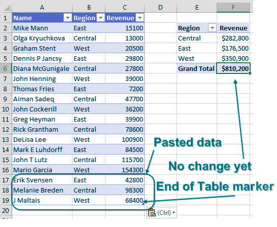
Go to the blank row below the table and paste. The new records pick up the formatting from the table. The angle-bracket-shaped End-of-Table marker moves to C19. But notice that the pivot table has not updated yet.
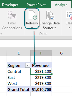
Click the Refresh button in the Pivot Table Tools Analyze tab. Excel adds the new rows to your pivot table.
Bonus Tip
Ctrl + T Helps VLOOKUP and Charts
In this figure, the VLOOKUP table is in E5:F9. Item A106 is missing from the table and the VLOOKUP is returning #N/A. Conventional wisdom says to add A106 to the middle of your VLOOKUP table so you don’t have to rewrite the formula.
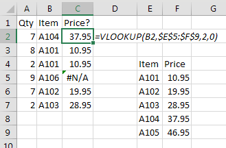
Instead, use Ctrl + T to format the lookup table. Note that the formula is still pointing to E5:F9; nothing changes in the formula.
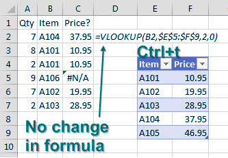
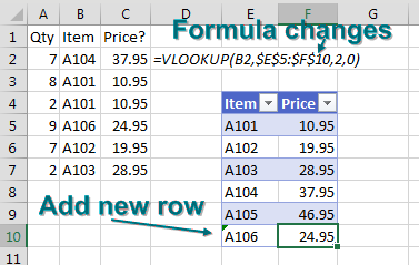
But when you type a new row below the table, it becomes part of the table and the VLOOKUP formula automatically updates to reflect the new range.
The same thing happens with charts. The chart on the left is based on A1:B5 which is not a table. Format A1:B5 as a table by pressing Ctrl + T. Add a new row. The row is automatically added to the chart.
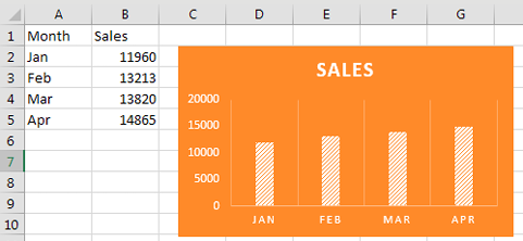
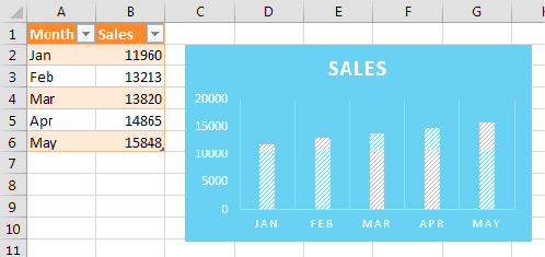
It is fairly cool that you can use Ctrl + T after setting up the pivot table, VLOOKUP, or chart, and Excel still makes the range expand.
Watch Video
- In the last episode, Ctrl + T made the pivot table source expand
- This also helps VLOOKUP and Charts and Data Validation
- Although it is slightly different in each
- Create your VLOOKUP then make the table a Ctrl + T table
- Remarkably the VLOOKUP formula will rewrite itself
- Build a chart. Make the source data a Ctrl + T table. Add new months.
- For Data Validation Source: Make it a table and then name the range without the heading
- Use the named range as the Validation Source
- Also mentioned in the episode: FORMULATEXT function for showing a formula
Video Transcript
Learn Excel for MrExcel Podcast, Episode 2002 – CTRL T Helps VLOOKUP
I'm podcasting this entire book, go ahead and subscribe to the playlist, top right hand corner, there's an I up there and welcome back to the MrExcel netcast. I'm Bill Jelen.
So yesterday's podcast we talked about how CTRL T makes your Pivot Table Data automatically grow. The other really amazing thing, here, is I have a VLOOKUP. So there's the VLOOKUP and you're seeing the FORMULA over here thanks for the FORMULA TEXT FUNCTION. I love FORMULA TEXT. It was brand new in Excel 2013. It lets me show you the FORMULA and the results side-by-side. Okay and you can see that this FORMULA is pointing to a Table here that's one, two, three, four, or five rows, , but there's something missing. So A106. Alright now here's the amazing thing I'm going to take this Table. This little VLOOKUP Table here. I'm going to do CTRL T, to make it into a real Table. My Table has headers and then, I'm going to come here and type A106, the missing item, outside of the range, and it's $88 and did you see that that? The FORMULA automatically rewrote itself to now go down through row F10. It didn't rewrite itself to refer to the Table, using Table nomenclature, , but it it simply worked .
Here's another example where CTRL T makes things better. Here's a chart, January through April, here's the Data, I'm going to CTRL T the Data and notice in all these cases the VLOOKUP, the chart, it was all there, just from a regular range and now when I add new Data, so here's May and we'll give it 15,000 it automatically grows. Alright, and when I look at the chart series, because I'm fascinated about how this works, the the chart series doesn't get rewritten in Table nomenclature, but it simply says, oh hey this is a Table we're going to extend from row five to row six. And here's another one. I picked this one up, this one's not in the book, this is a bonus. I picked this up at an amazing conference in Lucerne, Switzerland, called Trainer Tage. That's German for Trainer Days. These are, the the Trainer Tage Team, I was lucky enough to speak there for two years, Tanya Kuhn puts us on, and saw this amazing trick.
So we want to have a Data Validation List and we might be adding more things to the end of the Data Validation List. So, here's my list. I'm going to CTRL T to make it into a Table and then I'm going to very carefully name everything except for the heading. So I'll call it MyList ENTER. Right, so we just created a name there and then here we're going to go to Data and then it's drop-down, choose Data Validation. We're going to allow a List and the source is going to be =MyList ENTER. Alright, so now, what we should expect to see is Apple threw Fig would be there. Beautiful. Alright, but then when I come along and I type a new item, that End Of Table Marker is going to move down to the bottom of row 8, and remarkably, it's going to be in he list. Right, these are all great amazing side benefits of using Tables.
Alright now, of course I'm going to ask you to buy my book, but before I do that, I should give credit to Zach Barresse and Kevin Jones who wrote THE book on Excel Tables. Right, if you need to learn anything about Tables, or just see all the amazing stuff that comes about when you use Tables, check out this book from Zach and Kevin. Alright yeah, and then of course, I wish you to buy my book, so much knowledge in the palm of your hand. All of the tips from all of August and September podcasts. Right there. 10 bucks is an e-book, 25 bucks is a print book. Click the I in the top right hand corner.
Alright, so a recap here. In the last episode we use CTRL T to make the Pivot Table Source expand. It also helps VLOOKUP and Charts and Data Validation. It's slightly different in each, but you know, even after the VLOOKUP and the Charts are set up, you can, after the fact, make it into a Table and the VLOOKUP and the charts will expand. So create your VLOOKUP and then make the Table, the VLOOKUP Table of CTRL T Table and the FORMULA just rewrites itself. It's so cool. Or build a chart and then make it into a CTRL T Table and as you add new Data the Chart will automatically expand for Data Validation. Right now, this is from Tanya in Switzerland, make it a Table and then name the range without the heading, and then used the name range as the Validation Source. I also mentioned the Form Of The Text Function.
Alright now, when I ask people to send in their favorite tips, Tables were popular. Alright, Peter Albert, Snorri Iceland, Nancy Federici, Colin Michael, James Mead, KR Patel, Paul Payden and then a bunch of people suggested using OFFSET to create expanding ranges for dynamic charts. Charlie, Don, Francis and Cecilia. Tables now do the same thing in most cases, so you don't need OFFSET anymore. So, I actually took their ideas and threw them out, and put Tables in instead, but I still appreciate them sending their ideas in.
I appreciate you for stopping by. We'll see you next time for another netcast from MrExcel.
Download File
Download the sample file here: Podcast2002.xlsx
Title Photo: Free Photos / pixabay
