Create Easier-to-Understand Formulas with Named Ranges
December 01, 2021 - by Bill Jelen

Problem: How can I create easier-to-understand formulas?
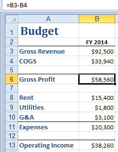
Strategy: It would be easier to understand the results if each component of every formula were named for what it represented and not just for the cell it came from. You can therefore use named ranges to make formulas easier to understand:
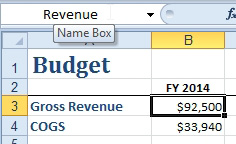
1. Select cell B3. In the Name box (the area to the left of the formula bar), type Revenue and press Enter.
2. Select cell B4. Click in the Name box, type COGS, and press Enter.
-
3. Clear the formula in B6. Reenter the formula and use the mouse to select the cells. Type =. Using the mouse, touch B3. Type -. Using the mouse, touch B4. Excel will enter the formula as =Revenue-COGS. This is easier to understand than a typical formula.
Gotcha: You need a lot of foresight to use this technique. In order to have this work automatically, you are supposed to be smart enough to create the range names before you enter the formula.
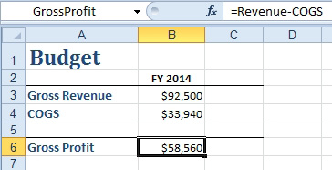
However, most people create a formula first and then decide to make the worksheet easier to understand. To assign range names after creating formulas, follow these steps:
1. Select Formulas, Define Name dropdown, Apply Names. Gotcha: Don’t click on the words Define Name; click on the dropdown icon to the right of Define Name.
2. Select all the names you want to apply and click OK.

Results: A formula like =B6-B11 will be updated to =GrossProfit-Expenses.
Additional Details: One advantage of named ranges: they are always treated as an absolute reference. You don’t need to add dollar signs to have the formula always point to that cell.
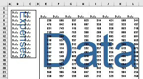
Problem: How can I see all named ranges at 39% zoom?
Set your zoom to 39% or less. Excel outlines and labels each named range.
This article is an excerpt from Power Excel With MrExcel
Title photo by Tim Mossholder on Unsplash
