Create an Amortization Table
February 09, 2022 - by Bill Jelen

Problem: I know it is easy to figure out a monthly payment using PMT. I would like to see my loan balance after each month’s payment. How can I build an amortization table?
Strategy: You can use PPMT and IPMT to build this amortization table. Here’s how:
1. In a blank section of the worksheet, add the column headings Payment, Date, Principal, Interest, and Balance.
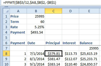
2. Ensure that the formula for Balance in the first row points to the price in B1.
-
3. In the next row of the table, enter the number 1 for Payment. Ctrl+drag the fill handle to fill in the proper number of payments.
4. Enter the first payment date for the Date. Right-click+drag the fill handle to the last row. When you release the mouse button, choose Fill Months.
5. Enter the PPMT function, using the proper absolute references, so that you can copy the function to column D to be used for IPMT. The syntax is
=PPMT(rate, per, nper, pv, [fv], [type]). The only difference from the PMT function is the addition of the period number as the second argument. In C8, type=PPMT(. The rate is B3/12, but after clicking on B3, press the F4 key to add the dollar signs. Type /12 and a comma. Click on the first payment number. Press the F4 key three times so that a dollar sign appears before the column number. Type a comma. Click on the Term in B2 and press F4. Type a comma. Type a minus sign and click on the price in B1. Press F4 and type the closing parenthesis. The whole formula is=PPMT($B$3/12,$A8,$B$2,-$B$1).

6. Copy this formula to the Interest Payment column. Edit the formula and change PPMT to IPMT. Use the F2 key or double click the cell in order to edit the formula. Alternatively, select the cell. Use the mouse to select the first P in PPMT in the formula bar. Type an I to change to IPMT.
7. For the Balance formula, use the previous balance minus this month’s principal payment.
8. Select the three cells that contain the principal, interest, and balance calculations. Double-click the fill handle to copy the formulas for all months.

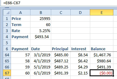
Additional Details: To test that the table is correct, scroll to the last row. You should see that the balance reaches zero with the last payment.
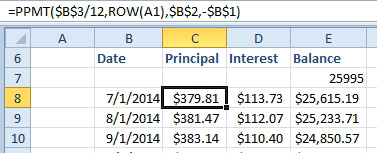
Alternate Strategy: Anytime that you have to enter the numbers 1 to nn for a formula, there is a cool alternative. Instead of putting the formulas in the worksheet, use ROW(A1) where the 1 needs to go. When you copy the formula down, it will change to ROW(A2) which will return a 2, and so on.

This article is an excerpt from Power Excel With MrExcel
Title photo by Danielle Cerullo on Unsplash
