Create a Year-Over-Year Report
December 27, 2022 - by Bill Jelen

Problem: I have two years of data by daily dates. I would like to see year-over-year sales by month.
Strategy: Amazingly, it takes only 10 mouse clicks to create this report. Follow these steps:
1. Select one cell in your data set.
2. Insert, Pivot Table, OK.
-
3. In the PivotTable Field List, choose Date and Revenue.
4. At this point, the Row Labels heading is selected. Move down one cell so that the cell pointer is on a date.
5. Choose Group Field. Months is already selected. Add Years. Click OK.
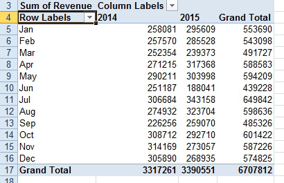
6. In the PivotTable Field List, drag Years from the Row Labels drop zone to the Column Labels drop zone. You will now have this report.

7. On the Design tab, open the Grand Totals dropdown and choose On For Columns Only which is the very strange way to delete the grand totals along the right side of the report.
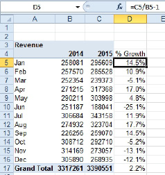
8. In D4, type
% Growth.9. In D5, type
=D5/C5-1. Do not use the mouse or arrow keys while entering this formula!10. Format D5 as a percentage with 1 decimal place.
11. Copy D5 down to all rows.
12. Select the Sum of Revenue heading. In the Analyze ribbon tab, click in the Active Field box and change the field name to “Revenue “ (with a space after the word Revenue.)
13. On the Analyze ribbon tab, click the Field Headers to prevent those from being shown in the report.

Gotcha: If you used the mouse in step 9, you will find that the percentage growth does not change as you copy it down. Go back and re-enter the formula, or follow the steps in Calculations Outside of Pivot Tables.
This article is an excerpt from Power Excel With MrExcel
Title photo by Clay Banks on Unsplash
