Copy a VLOOKUP Across Many Columns
April 15, 2022 - by Bill Jelen

Problem: I’ve entered a VLOOKUP for January. I need to copy the formula across eleven additional columns.
Strategy: There are a few things you can do to make this process simpler:
- Press F4 three times when entering the lookup value. This will change A2 to $A2. The single dollar sign ensures the lookup will always reach back to column A for the lookup value.
- Press F4 once when entering the lookup table. This will change the lookup table to have four dollar signs, $P$4:$AB$227. Alternatively, name the lookup table first, then you won’t have to use dollar signs. See Consider Naming the Lookup Table.
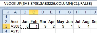
The big problem is the third argument. I find that I end up editing each copied formula to change to 2 to a 3, then a 4, then a 5, and so on.
I have two solutions for this.
- Enter a temporary row with the numbers 2 through 13 stretching across the row. This row could be above the table you are trying to build. Then, instead of specifying 2 as the column to return, you can point to B1 and press F4 twice to change it to B$1.

- The other solution is to replace the
,2,with,COLUMN(B1),. TheCOLUMNfunction returns the column number of the given cell. Since B1 is in the second column, it will return a 2. I like to say that this is the world’s geekiest way of writing the number 2. However, the advantage is that when you copy this formula to the right, the reference inside theCOLUMNfunction will automatically change to C1, which is in column 3. Using this method allows you to enter one formula without having the temporary values in row 1.

Additional Details: The second method will slow your VLOOKUPs down, as Excel has to calculate the COLUMN function in every row of your lookup table.
Alternate Strategy: You can speed up the VLOOKUPs if you add one column of MATCH functions and then use 12 columns of the incredibly speedy INDEX function. Before you can do this, though, you need to learn about these two incredibly arcane functions.
This article is an excerpt from Power Excel With MrExcel
Title photo by Linus Nylund on Unsplash
