Convert Your Data to a Table Before Adding Records
December 01, 2022 - by Bill Jelen

Problem: I have 100 new records to paste below the original data that is in the pivot table. How do I do that?
Strategy: There are two solutions. I recommend the second one.
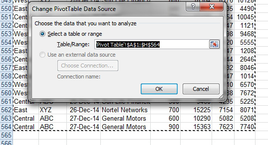
- Paste the new data below your original data. Select a cell in the pivot table. Choose the Change Data Source icon (see Figure 837 above).
- Select a cell in the original data set. Press Ctrl+T to define the data as a table. Paste new data below the original data. The Data Source is automatically updated. Simply click the Refresh button to incorporate the new records.
The table feature began in Excel 2003 as a List. In Excel 2007, it was renamed to be a Table, creating confusion between the Data Table found in the What-If tools and the Format as Table command on the Home tab.
The Table applies some interesting formatting. The Table adds Filter dropdowns. The Table makes it easier to enter formulas. But the most valuable feature of the table is to have the pivot table data range automatically grow as you add new rows to the underlying data.
Here is an example.
Currently, the pivot table uses rows 1:564 of data.

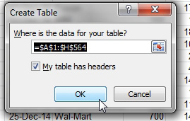
Select a cell in that data and press Ctrl+T. Confirm the location of the table.

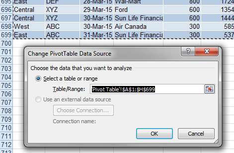
When you paste 2015 Q1 data below the original data, the table definition automatically changes. The other thing that updates is the range used for the PivotTable Data Source. You no longer have to visit this dialog, as it is already updated.

This still counts as a change to the underlying data, so you have to click the Refresh button to update the pivot table.
This article is an excerpt from Power Excel With MrExcel
Title photo by Markus Winkler on Unsplash
