Convert a Table of Numbers to a Visualization

August 09, 2023 - by Bill Jelen

Problem: My manager’s eyes glaze over when he sees a table of numbers. Is there anything I can do to help him spot trends in the data?

Five weekdays across the top, sales reps down the side, and numbers in the middle — Figure 1258. Help your manager to understand this data.

Strategy: You can use one of the three new data visualization tools on the Conditional Formatting menu: data bars, color scales, and icon sets.

Adding a data bar to a range adds an in-cell bar chart to each cell. You can see which cells have the largest values by seeing which cells have the most color.

To add data bars, you select a range of numbers and then select Home, Conditional Formatting, Data Bars, choose a color. Excel offers six gradients and six solid. You can choose More Rules to add any of 16 million colors.

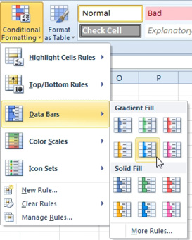
Choose, Home, Conditional Formatting, Data Bars, Blue. — Figure 1259. Choose a color for the data bars

Below, you can see that Wednesday is the busiest day. Calls fall of on Friday for everyone except Missy. Missy is consistently the strongest performer.

Every numbers gets a tiny bar starting from the left edge of the cell. The largest numbers have longer bars. — Figure 1260. Easily spot trends in the data.

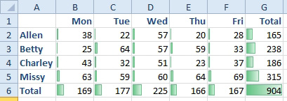
Gotcha: You should not include any total cells in your selection when applying conditional formatting. The relative size of the totals would make all the detail numbers receive small bars. Below, the 904 in cell G6 makes all the cells in B2:F5 look relatively the same.

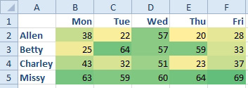
When you include a total row, total column, or even worse, a grand total in the data bar range, all of the individual numbers are too small and get hardly any color. — Figure 1261. Don’t include totals in a visualization.

Additional Details: You can use color scales to apply a mix of colors to a range. Excel offers built-in three-color scales such as red-yellow-green as well as two-color scales. The two-color scales look better than three-color scales when printed in monochrome. You can also use More Rules to design your own color scheme. Below, the largest numbers are in the darker green, and the smallest numbers are in the lighter yellow.

Weekdays across the top, names down the left, and values in the middle. Add a color scale. The largest numbers have the darkest shading. — Figure 1262. Each cell is lighter or darker based on size.

The final new visualization is icon sets.

In Excel 2010, there are 20 sets of icons. Some have three symbols, others have four, and some have five.

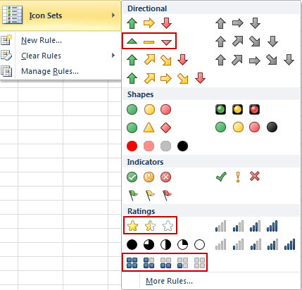
Home, Conditional Formatting, Icon Sets leads to a flyout with 20 different pre-built icons. Three of these were added in Excel 2010 - one has an up arrow, a yellow dash, and a down arrow to indicate up, flat, down. — Figure 1263. Twenty icon sets are available.

Note that for many of these sets you need to print in color in order for the reader to differentiate the symbols. If you are printing in monochrome, the arrows or power bars are good choices.

After you choose an icon set, Microsoft will display the icon at the left of each cell. Since numbers are usually right-aligned, the number from B2 and the icon from C2 are too close together and many will think that they go together.

I’ve begun using Ctrl+1 to visit the Format Cells dialog. On the Alignment tab, use a horizontal alignment of Right (Indent). You can then increase the indent to 2 or 3 to move the numbers closer to their icons.

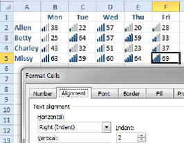
An icon set with cell phone power bars as the icons. Because the icons are always left-aligned, use Format Cells, Alignment, Right (Indent) and indent by 2 characters to move the number closer to the icon. — Figure 1264. Indent numbers to move them closer to the icons.

The icons won’t respond to the horizontal alignment of the cell, unless you use Home, Conditional Formatting, Manage Rules, Edit Rule, Show Icon Only. Ironically, when you use this setting, the icon responds to the Left, Center, and Right Align buttons in the Home ribbon!

This article is an excerpt from Power Excel With MrExcel

Title photo by Lukas Blazek on Unsplash