Control Values for Each Icon

August 10, 2023 - by Bill Jelen

Problem: I applied an icon set. They are adding green checkmarks to cells that are not in the best quality range.

Strategy: By default, Microsoft finds the range of values in your range, divides it by the number of icons in the set (three, four, or five) and creates equal ranges.

Data with the three shapes icon set. Green checkmarks for the big numbers. Yellow exclamation points for middle numbers, and red X for the lowest numbers. — Figure 1265. 50-67 gets a red X, 84 and up gets a checkmark.

Excel does a quick calculation to get some icons drawn in. If you have defined limits of acceptable values, you can override the defaults to define your own ranges.

Add the icon set. Select the cells that contain the icon. Go to Home, Conditional Formatting, Manage Rules. Select the one rule and click Edit Rule.

When an icon set has three symbols, the top symbol is for when value is greater than or equal to 67 percent. The middle icon is for greater than or equal to 33 percent. Drop-downs are available to change the greater than or equal to choice to an equals sign. The Type drop-downs are Percent, Percentile, Number, or Formula. — Figure 1266. The default is by percent.

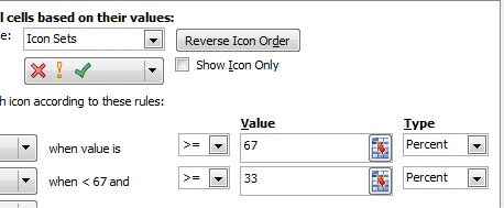
In the sample workbook for this topic, the range of data is 50 to 100. Excel split that range of values into values. Anything of 84 or above gets the green checkmark. Note that because the data is skewed high, 57% of the values in the entire data set are getting green checkmarks.

The Type dropdown in the figure above offers Percent, Percentile, Number, and Formula.

If you would use Percentile, Excel would redefine the ranges. About 40 of the 120 values would get each icon. With this data set, 80-90 gets the yellow marker. 79 and below is red, 91 and above is green.

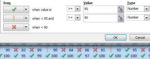
The Type that I use frequently is Number. When using Number, you can define it so that scores of 95 and above get green, 90-94 are yellow and everything else is failing with red.

Edit the icon set dialog so the green checkmark is for greater than or equal to 95 number. The middle icon is for greater than or equal to 90 number. The last icon then defaults to less than 90. — Figure 1267. Define the ranges to use.

To use the Formula, you have to type a formula that will result in a number. For example, =AVERAGE($B$2:$M$11)+STDEV.P($B$2:$M$11) will calculate a point that is one standard deviation greater than the mean.

This article is an excerpt from Power Excel With MrExcel

Title photo by Possessed Photography on Unsplash