Combine Two Lists Using VLOOKUP
April 28, 2022 - by Bill Jelen

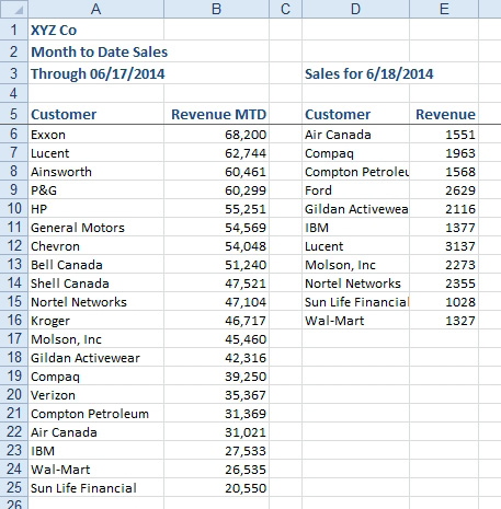
Problem: I have a list of month-to-date sales by customer. My co-worker just sent me a list of sales for yesterday. I need to combine and merge these lists.

This is a 3-step process:
- Do a
MATCHor aVLOOKUP(,,1,)on the second list to find new customers. Add the new customers to the original list with previous sales of 0. - Now that the first list contains a superset of customers in either list, do a
VLOOKUPon the first list to get the sales from the second list. - Add previous sales to new sales and convert to values. You can now delete the new list.
- When you want to figure out if a customer in column D is already in column A, most people will do
=VLOOKUP(D6,A6:A25,1,False). This will either show the customer name or #N/A. In this case, you are interested in the #N/A records.
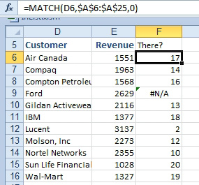
However, now that you’ve read about MATCH, you can just as easily use MATCH to find which customers are in the other list. Use =MATCH(D6,$A$6:$A$25,0). In the figure below, all of the customers in column D have a match except Ford.
Any customers with #N/A are new customers and need to be added to the list of customers in column A. If you get a few #N/A values, sort by column F to bring the new customers together. Copy just the customer name and paste to the bottom of the list in column A. Enter $0 as the sales in column B for the new customers.

In the current example, only Ford is new, so you can copy Ford from D9 and paste to A26. Enter zero in B26. In real life, though, you will have a several customers who are new. Copy and paste below the first customer in A. Add zero to all the corresponding cells in B.
You’ve now completed the first of three steps. The next step is to add the real VLOOKUP to the first list.
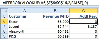
=VLOOKUP(A6,$E$6:$F$16,2,FALSE) would return a mix of revenue values and #N/A errors. When an existing customer had no revenue on June 18, the result of the VLOOKUP will be #N/A. You can use the new IFERROR function to replace those #N/A values with zeroes.
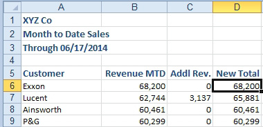
Insert two new columns before column D. Label these temporary columns Addl Rev and New Total.
The formula in the new C6 is =IFERROR(VLOOKUP(A6,$F$6:$G$16,2,FALSE),0). Copy that formula down to row 26.

If you want to check your work, use AutoSum to add a total at the bottom of column C and the bottom of column G. Both totals should match.
That completes step two of three steps. The final step is to combine revenue from column B and column C.
In D6 enter a formula of =B6+C6. Copy this formula down.

Copy D6:D26. Select B6 and Paste Values.
Gotcha: Don’t worry that column D is showing a higher value than it should. Column D is still adding the current day’s revenue to the new total in B. You will be deleting column D very soon. If you don’t want column D to ever show a wrong value, you could copy D and paste values on top of itself first.
Change the date in A3 to indicate that the report has data through 6/18.
Delete the temporary columns C through H.
It looks like the original data was sorted by descending revenue. Choose cell B6 and click the ZA button on the Data tab of the ribbon.
This process of comparing and combining two lists using VLOOKUP is a staple of data analysis. There is a faster and easier way to do this.
See Use a Pivot Table to Compare Two Lists.
This article is an excerpt from Power Excel With MrExcel
Title photo by Torbjørn Helgesen on Unsplash
