Coerce an Array of Dates from 2 Dates
July 05, 2022 - by Bill Jelen

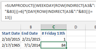
Problem: I have a start date in A and an end date in B. I need to see how many days between those two dates fell on Friday the 13th.
Strategy: This formula came from the MrExcel.com message board. It is one of the coolest formulas that I have ever seen. This one formula will replace 108,000 formulas. While this formula is figuring out the number of Friday the thirteenths, you can use this method any time you need to compare every date between two dates to something. I will show you the formula first and then explain it in detail.

The explanation here is about row 2. The same concept applies to row 3.
1. Remember that dates are really stored as the number of days elapsed since January 1, 1900. The date in A2 is really stored as 42045.
-
2. The date in B2 is really stored as 42056.
3. Concatenate those two numbers with a colon in between. You get 42045:42056. This is actually a valid Excel reference. It refers to all of the rows from 42045 to 42056.
4. Take the text from #3 and put it inside an
INDIRECT(42045:42056)function. Since that is a valid reference, you now are referencing a range of all the rows from 42045 to 42056.5. Use the ROW() function on the reference from step 4. You now have an array of row numbers:
{42045; 42046; 42047; 42048; 42049; 42050; 42051; 42052; 42053; 42054; 42055; 42056}. Note that this array is relatively small. Down in row 3, there will be 18,000 numbers in the array. For the rest of the steps, stop thinking about those as numbers and start thinking about them as dates.6. Take the
WEEKDAY()of each number in the array from #5. You get{3; 4; 5; 6; 7; 1; 2; 3; 4; 5; 6; 7}. In this version ofWEEKDAY, Sunday is 1 and Friday is 6.7. Test to see if the results of step 6 are equal to 6 which means Friday. You now have an array of True/False values:
{False; False; False; True; False; False; False; False; False; False; True; False}.8. Go back to that array from step 5 and put it in the DAY() function. This will return an array of only the day portion of the date:
{10; 11; 12; 13; 14; 15; 16; 17; 18; 19; 20; 21}.9. Take the array from 8 and test to see if it is 13.
{False; False; False; True; False; False; False; False; False; False; False; False}.10. Multiply the array from 7 by the array from 9. If both have a TRUE in the same position you will get a 1, otherwise a 0. You get:
{0; 0; 0; 1; 0; 0; 0; 0; 0; 0; 0; 0}.11. Sum all of the 1’s from step 10 using
SUMPRODUCT. In this case, you get a 1 as the total. In the case of row 3, you get 84 occurrences of Friday the 13th in a span of 49 years.
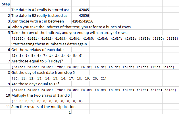
It might help to picture the calculation happening in Excel.

Picture the calculation for C3. instead of 12 items in each array, there are 18,000 items in each array. That one formula takes two date cells and coerces it into several arrays of 18,000 items each.
If you find this type of formula interesting, check out my other book, Excel Gurus Gone Wild.
This article is an excerpt from Power Excel With MrExcel
